Learning Partially Observable Deterministic Action Models

1 Introduction

Autonomous agents have limited prior knowledge of their actions' preconditions and effects when they explore new domains. They can act intelligently if they learn how actions affect the world and use this knowledge to respond to their goals. This is important when their goals change because then they can reason about their actions instead of trying them in the world.

Learning actions' effects and preconditions is difficult in partially observable domains. The world state is not known completely, actions' effects mix with each other, and it is hard to associate change in one feature with a specific action or situation. Thus, it is not surprising that work so far has been limited to fully observable domains (e.g., [Wang, 1995; Pasula et al., 2004]) and to hill-climbing (EM) approaches that have unbounded error in deterministic domains (e.g., [Ghahramani, 2001; Boyen et al., 1999]).

This paper presents an approach called SLAF (Simultaneous Learning and Filtering) for exact learning of action's effects and preconditions in partially observable deterministic domains. This approach determines a set of possible transition relations, given a sequence of actions and partial observations. It is online, and updates a logical formula that models the possible transition relations and world states with every time step. It finds exactly those transition relations when actions are STRIPS (i.e., no conditional effects) or they map states 1:1.

Our algorithms take polynomial time in the number of features, n, and the number of time steps, T, for many cases. Their exact complexity varies with properties of the domain. For example, the overall time for learning STRIPS actions' effects is O(T · n). For other cases the update per time step takes linear time in the representation size. We can bound this size by O(nk ) if we approximate the representation with a k-CNF formula, yielding an overall time of O(T · nk ) for the entire algorithm.

Our experiments verify these theoretical results and show that our algorithms are faster and better qualitatively than related approaches. For example, we can learn STRIPS actions' effects in domains of > 100 features exactly. In contrast, work on learning in Dynamic Bayesian Networks (e.g., [Boyen et al., 1999]), reinforcement learning in POMDPs (e.g., [Littman, 1996]), and Inductive Logic Programming (ILP) (e.g., [Wang, 1995]) either approximate the solution with unbounded error for deterministic domains, or take time Ω(22n ) (thus, are inapplicable in domains larger than 10 features). Section 7 provides a comparison with these and other works.

Our technical advance for deterministic domains is important for many applications such as automatic software interfaces, internet agents, virtual worlds, and games. Other applications, such as robotics, human-computer interfaces, and program and machine diagnosis can use deterministic models as approximations. Finally, understanding the deterministic case better can help us develop better results for stochastic domains.

In the following, Section 2 defines SLAF precisely, Section 3 provides a deduction-based exact SLAF algorithm, Section 4 presents tractable model-update algorithms, Section 5 gives sufficient conditions and algorithms for keeping the model representation compact (thus, overall polynomial time), and Section 6 presents experimental results.

2 SLAF Semantics

We define our SLAF problem with the following formal tools, borrowing intuitions from work on Bayesian learning of Hidden Markov Models (HMMs) [Ghahramani, 2001] and Logical Filtering [Amir and Russell, 2003].

A transition system is a tuple 〈P, S, A, R〉, where

• P is a finite set of propositional fluents;
• S ⊆ Pow(P) is the set of world states;
• A is a finite set of actions;
• R ⊆ S ×A× S is the transition relation.

Thus, a world state, s ∈ S, is a subset of P that contains propositions true in this state, and R(s, a, s′ ) means that state s′ is a possible result of action a in state s. Our goal in this paper is to find R, given known P, S, A, and a sequence of actions and partial observations (logical sentences on any subset of P).

A transition belief state is a set of tuples 〈s, R〉 where s is a state and R a transition relation. Let R = P ow(S× A× S) be the set of all possible transition relations on S, A. Let S = S × R. When we hold a transition belief state ρ ⊆ S we consider every tuple 〈s, R〉 ∈ ρ possible.

For example, consider the situation presented in Figure 1. There, we have two rooms, a light bulb, a switch, an action of flipping the switch, and an observation, E (we are in the east room). The real states of the world, s2, s2′ (shown in the top part), are unknown to us.

The bottom part of Figure 1 demonstrates how our knowledge evolves after performing the action sw-on. ρ1, ρ2 are our respective transition belief states. In ρ1 we know that the possible world states are s2, s1, or s3 (s1, s3 are arbitrary world states), with R2, R1, and R3, their respective transition relations. ρ2 is the resulting transition belief state after action sw-on. Action sw-on takes state s2 to s2′ according to transition relation R2, so 〈s2′ ,R2〉 is a pair ρ2. Similarly, it takes state s1 to one of s1′ , s1′′ according to transition relation R1, and it takes s3 to s3′ according to R3. Thus, 〈s1′ ,R1〉, 〈s1′′ ,R1〉, 〈s3′ ,R3〉 are in pair ρ2. Finally, observing E eliminates the pair 〈s3′ ,R3〉 from ρ2, if E is false in s3′ .

Definition 2.1 (SLAF Semantics) Let ρ ⊆ S be a transition belief state. The SLAF of ρ with actions and observations 〈aj, oj〉1≤j≤t is defined by

1. SLAF[a](ρ) =
2. {〈s′ ,R〉 | 〈s, a, s′ 〉 ∈ R, 〈s,R〉 ∈ ρ};
3. SLAF[o](ρ) = {〈s,R〉 ∈ ρ | o is true in s};
4. SLAF[〈aj, oj〉i≤j≤t ](ρ) = SLAF [〈aj , oj 〉i<j≤t ](SLAF [oi ](SLAF [ai ](ρ))).

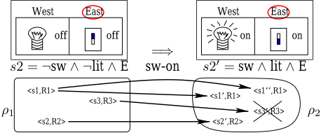
Step 1 is progression with a, and Step 2 filtering with o.

We assume that observations (and observation model relating observations to state fluents) are given to us as logical sentences over fluents after performing an action. They are denoted with o. When actions can be inexecutable or may fail, it is useful to assume that P contains a special boolean fluent, OK, whose value is the success of the last action attempted.

Transition belief state ρ generalizes version spaces (e.g., [Wang, 1995]) as follows: If the current state, s, is known, then the version space's lattice contains the set of transition relations ρs = {R | 〈s,R〉 ∈ ρ}. It also generalizes belief states: If the transition relation, R, is known, then the belief state (set of possible states) is ρR = {s | 〈s,R〉 ∈ ρ} (read ρ restricted to R), and Logical Filtering [Amir and Russell, 2003] of belief state σ and action a is equal to (thus, we define it as)

3 SLAF via Logical Inference

Learning transition models using Definition 2.1 directly is intractable because it takes space Ω(22|P| ) in many cases. Instead, in this section we represent transition belief states more compactly (sometimes) using logic, and compute SLAF using general purpose logical inference.

We represent every deterministic transition relation, R, with a language, L, of propositions aFG whose meaning is "If G holds, then F will hold after executing a". We have aFG ∈ L for every action a ∈ A, F a literal (possibly negated proposition) from P, and G a complete term over P (a conjunction of literals from P such that every fluent appears exactly once). We call F, G the sets of effects, F, and preconditions, G, respectively. Thus, we have 2|P| · 2|P| · |A| new propositional variables (in Section 5 we decrease this number).

Define ϕR, the logical theory that represents R, by ϕ0R = {aFG ∈ L | ∀〈s, a, s′ 〉 ∈ R, s |= G ⇒ s′ |= F} and ϕR = ϕ0R ∪ {¬aFG | aFG ∈ L \ ϕ0R}.

Some intuitive properties hold for this representation. ϕR is a complete theory for every R (a sentence or its negation is always implied from ϕR). Also, ϕR |= ¬aFG ⇔ a¬F G , for every F ∈ F,G ∈ G.

Thus, for every transition belief state ρ we can define a theory in L(L ∪ P) that corresponds to it: ϕρ = ∨〈s,R〉∈ρ (s ∧ ϕR). Similarly, for every theory ϕ in L(L ∪ P) we define a transition belief state ρϕ = {〈s,R〉 | s ∈ S, s∧ϕR |= ϕ}, i.e., all the state-transition pairs that satisfy ϕ. We say that theory ϕ is a transition belief formula, if ϕρϕ ≡ ϕ (note: ρϕρ = ρ always holds).

For a deterministic (possibly conditional) action, a, define the effect model of a for time t to be

where at asserts that action a occurred at time t, and we use the convention that ϕt is the result of adding subscript t to every fluent symbol of ϕ. The first part of (1) says that if a executes at time t, and it causes l when G holds, and G holds at time t, then l holds at time t + 1. The second part says that if l holds after a's execution, then it must be that alG holds, with G corresponding to the current state. These two parts correspond to effect axioms and explanation closure axioms used in Situation Calculus.

Now, we are ready to describe our zeroth-level algorithm (SLAF0) for SLAF of a transition belief formula. Denote by CnV (ϕ) the set of consequences of ϕ that are in vocabulary V , and let Lt+1 = Pt+1 ∪ L the vocabulary that includes only fluents of time t + 1 and effect propositions from L. At time t we apply progression for the given action a and current transition belief formula, ϕt, and then apply filtering with the current observations:

We can implement CnV (ϕ) using consequence finding algorithms, such as resolution and some of its variants (e.g., [Simon and del Val, 2001]). The following theorem shows that this formula-SLAF algorithm is correct and exact.

Theorem 3.1 For ϕ transition belief formula, a action,

Our zeroth-level algorithm may enable more compact representation, but it does not guarantee it, nor does it guarantee tractable computation. In fact, no algorithm can maintain compact representation or tractable computation in general. SLAF is NP-hard because Logical Filtering is NP-hard [Eiter and Gottlob, 1992] even for deterministic actions. Also, any representation of transition belief states that uses poly(|P|) propositions grows exponentially (in the number of time steps and |P|) for some starting transition belief states and action sequences.

4 Efficient Model Update

Learning world models is easier when SLAF distributes over logical connectives. The computation becomes tractable, with the bottleneck being the time to compute SLAF for each part separately. In this section we examine when such distribution is possible, and present a linear-time algorithm that gives an exact solution in those cases (and a weaker transition belief formula otherwise).

Distribution properties that always hold for SLAF follow from set theoretical considerations and Theorem 3.1: Corollary 4.1 For ϕ, ψ transition belief formulae, a action,

Stronger distribution properties hold for SLAF whenever they hold for Logical Filtering.

Theorem 4.2 Let ρ1, ρ2 be transition belief states. SLAF [a](ρ1 ∩ ρ2) = SLAF [a](ρ1 ∩ ρ2) iff for every R Filter[a](ρR1 ∩ ρR2 ) = Filter[a](ρR1 ) ∩ Filter[a](ρR2 ).

We conclude the following corollary from Theorems 3.1, 4.2 and theorems in [Amir and Russell, 2003].

Corollary 4.3 For ϕ, ψ transition belief formulae, a action, SLAF [a](ϕ∧ψ) ≡ SLAF [a](ϕ)∧SLAF [a](ψ) if for every relation R in ρϕ,ρψ one of the following holds:

1. a in Rmaps states 1:1
2. a has no conditional effects (and we know if it fails), and ϕ ∧ ψ includes all its prime implicates.
3. The state is known for R: for at most one s, 〈s, R〉 ∈ ρϕ ∪ ρψ.

Figure 2 presents Procedure Factored-SLAF, which computes SLAF exactly when the conditions of Corollary 4.3 hold. Consequently, Factored-SLAF returns an exact solution whenever our actions are known to be 1:1. If our actions have no conditional effects and their success/failure is observed, then a modified Factored-SLAF can solve this problem exactly too (see Section 5).

If we pre-compute (and cache) the 2n possible responses of Literal-SLAF, then every time step t in this procedure requires linear time in the representation size of ϕt, our transition belief formula. This is a significant improvement over the (super exponential) time taken by a straightforward algorithm, and over the (potentially exponential) time taken by general-purpose consequence finding used in our zeroth-level SLAF procedure above.

Theorem 4.4 Step-SLAF(a, o, ϕ) returns a formula ϕ′ such that SLAF[a, o](ϕ) |= ϕ′ . If every run of LiteralSLAF takes time c, then Step-SLAF takes time O(|ϕ|c). Finally, if we assume one of the assumptions of Corollary 4.3, then ϕ′ ≡ SLAF[a, o](ϕ).

We can give a closed-form solution for the SLAF of a belief-state formula (a transition belief formulae that has no effect propositions aFG). This makes procedure Literal-SLAF tractable, and also allows us to examine the structure of belief state formulae in more detail.

PROCEDURE Factored-SLAF(〈ai, oi〉0<i≤t ,ϕ)

∀i, ai action, oi observation, ϕ transition belief formula.

1. For i from 1 to t do,
2. (a) Set ϕ← Step-SLAF(oi,ai,ϕ).
3. (b) Eliminate subsumed clauses in ϕ.
4. Return ϕ.

PROCEDURE Step-SLAF(o,a,ϕ)

o an observation formula in L(P), a an action, ϕ a transition belief formula.

1. If ϕ is a literal, then return o∧Literal-SLAF(a,ϕ).
2. If ϕ = ϕ1 ∧ ϕ2, return Step-SLAF(o,a,ϕ1)∧StepSLAF(o,a,ϕ2).
3. If ϕ = ϕ1 ∨ ϕ2, return Step-SLAF(o,a,ϕ1)∨StepSLAF(o,a,ϕ2).

PROCEDURE Literal-SLAF(a,ϕ)

• a an action, ϕ a proposition in Lt or its negation.
• Return CnLt+1 (ϕt ∧ at ∧ Teff(a, t)).

Figure 2: SLAF using distribution over ∧, ∨

Theorem 4.5 For belief-state formula ϕ ∈ L(P), time t, action a, Ca = ∧G∈G,l∈F (alG ∨ a¬l G ), and G1, ..., Gm ∈ G all the terms in G such that Gi |= ϕ,

PROOF SKETCH We follow the characterization offered by Theorem 3.1 and Formula (1). We take ϕt ∧ at ∧ Teff(a, t) and resolve out the literals of time t. This resolution is guaranteed to generate a set of consequences that is equivalent to CnLt+1 (ϕt∧at∧Teff(a, t)). Assuming ϕt ∧ at, Teff(a, t) is logically equivalent to Teff(a, t)|ϕ = ∧l∈F,G∈G,G|=ϕ((alG ∧ Gt) ⇒ lt+1) ∧ ∧l∈F,G∈G,G|=ϕ(lt+1 ⇒ (Gt ⇒ alG)). This follows from two observations. First, notice that ϕt implies that for any G ∈ G such that G ̸|= ϕ we get Gt ⇒ alG and (alG ∧ Gt) ⇒ lt+1 (the antecedent does not hold, so the formula is true). Second, notice that, in the second part of the original Teff(a, t), (∨G∈G,G|=ϕ(alG ∧Gt)) is

equivalent (assuming ϕ) to (∧G∈G,G|=ϕ(Gt ⇒ alG)). Now, resolving out the literals of time t from ϕt ∧at ∧ Teff(a, t)|ϕ should consider all the resolutions of clauses (Gt is a term) of the form alG ∧ Gt ⇒ lt+1 and all the clauses of the form lt+1 ⇒ (Gt ⇒ alG) with each other. This yields the equivalent to

because to eliminate all the literals of time t we have to resolve together sets of clauses with matching Gi's such that ϕ |= ∨i≤n Gi. The formula above encodes all the resulting clauses for a chosen set of G1, ...,Gm and a chosen set of literals l1, ..., lm. The reason for including (a¬li Gi ∧¬aliGi ) is that we can always choose a clause with Gi, li of a specific type (either one that includes ¬alG or one that produces a¬l G .

Finally, we get the formula in our theorem because aFG ≡ ¬a¬F G (G characterizes exactly one state in S), and the fact that there is one set of G1, ...,Gm that is stronger than all the rest (it entails all the rest) because G1, ...,Gm are complete terms. This set is the complete fluent assignments Gi that satisfy ϕ.

A consequence of Theorem 4.5 is that we can implement Procedure Literal-SLAF using the equivalence

Notice that the computation in Theorem 4.5 for ϕ = l a literal is simple because G1, ...,Gm are all the complete terms in L(P) that include l.

5 Compact Model Representation

In Theorem 4.5, m could be as high as 2|P| , the number of complete terms in G. Consequently, clauses may have exponential length (in n = |P|) and there may be a super-exponential number of clauses in this result.

In this section we restrict our attention to STRIPS actions [Fikes et al., 1972], and provide an overall polynomial bound on the growth of our representation, its size after many steps, and the time taken to compute the resulting model. STRIPS is a class of actions that has been at the focus of interest for the area of AI planning and execution for many years. It includes deterministic, unconditional (but sometimes not executable) actions.

5.1 Actions of Limited Effect

In many domains we can assume that every action a affects at most k fluents, for some small k > 0. It is also common to assume that our actions are STRIPS, and that they may fail without us knowing, leaving the world unchanged. Those assumptions together allow us to progress SLAF with a limited (polynomial factor) growth in the formula size.

We use a language that is similar to the one in Section 3, but which uses only action propositions alG with G being a fluent term of size k (instead of a fluent term of size n in G). Semantically, all1∧...∧lk ≡ ∧lk+1,...,ln all1∧...∧ln .

Theorem 5.1 Let ϕ ∈ L(P) be a belief-state formula, t time, and a a STRIPS action with ≤ k fluents affected or in the precondition term. Let Gk be the set of all terms of k fluents in L(P) that are consistent with ϕ. Then,

The proof (omitted) uses two insights. First, if a has only one case in which change occurs, then every clause in Theorem 4.5 is subsumed by a clause that is entailed by SLAF[a](ϕt), has at most one aliGi per literal li (i.e., li ̸= lj for i ̸= j) and Gi is a fluent term (has no disjunctions). Second, every alG with G term is equivalent to a formula on alGi with Gi terms of length k, if a affects only k fluents.

Thus, we can encode all of the clauses in the conjunction using a subset of the (extended) action effect propositions, alG, with G being a term of size k. There are O(nk ) such terms, and O(nk+1 ) such propositions. Every clause is of length 2k, with the identity of the clause determined by the first half (the set of action effect propositions). Consequently, SLAF[a](ϕt) takes O(nk2+k ·k2 ) space to represent using O(nk2+k ) clauses of length ≤ 2k.

5.2 Always-Executable Actions

Many times we can assume that our actions are always executable. For example, our sequence of actions does not include action failures when this sequence is chosen by a knowledgeable agent (e.g., a human) that has better observations than we do.

We use a language that is similar to the one in Section 3, but which uses only action propositions al (l always holds after executing a) and al ◦ (l is not affected by a). Semantically, al ≡ ∧l1,...,ln all1∧...∧ln , and

We assume that transition-belief formula ϕ is fluentfactored, i.e., it is the conjunction of ϕf such that each ϕf concerns only one fluent, f , and actions' effects on it. Also, for every f , ϕf ≡ (¬f ∨explf )∧(f ∨expl¬f )∧Af , with explf , expl¬f , Af formulae over action propositions af , a¬f , and af◦ (possibly multiple different actions). We call this format fluent-factored. The intuition here is that explf and expl¬f are all the possible explanations for f being true and false, respectively. Also, Af holds knowledge about actions' effects on f, knowledge that does not depend on f's current value. For example, if we know nothing about actions that affect f (e.g., when we start our exploration), then ϕf = (¬f ∨ TRUE) ∧ (f ∨ TRUE) ∧ TRUE.

With this representation, SLAF[a](ϕf) is

A similar formula holds for observations.

This contributes to a much simpler algorithm, AESTRIPS-SLAF, that we present in Figure 3. It computes SLAF of a fluent-factored transition belief state in this form with a sequence of actions and observations.

Theorem 5.2 Let ϕ be a fluent-factored transition belief formula, and assume a1, ..., aT are always-executable STRIPS actions, and o1, ..., oT are observation terms.

PROCEDURE AE-STRIPS-SLAF(〈ai, oi〉0<i≤T ,ϕ) ai actions, oi observations, ϕ = ∧f∈P ϕf fluent-factored with ϕf = (¬f ∨ explf ) ∧ (f ∨ expl¬f ) ∧ Af .

• (a) Set ϕf ← (¬f ∨ (af ∨ (af◦ ∧ explf ))) ∧ (f ∨ (a¬f ∨ (af◦ ∧ expl¬f ))) ∧ Af .
• For every f ∈ P do: For i from 1 to T do,
• (b) If oi |= f (we observed f), then set ϕf ← (¬f ∨ TRUE) ∧ (f ∨ FALSE) ∧ Af ∧ explf .
• (c) If oi |= ¬f (we observed ¬f), then set ϕf ← (¬f ∨ F ALSE) ∧ (f ∨ T RUE) ∧ Af ∧ expl¬f .
• Eliminate subsumed clauses in ϕ = ∧f∈P ϕf . 3. Return ϕT = ϕ.

Figure 3: SLAF with always-executable STRIPS.

Then, Procedure AE-STRIPS-SLAF(〈ai, oi〉0<i≤t ,ϕ) returns ϕT ≡ SLAF[〈ai, oi〉0<i≤t ](ϕ0) in time O(T · |P|), and |ϕT | ≤ O(T · |P|).

The reason for the space bound on the end formula |ϕT | is that at every time step we increase the size of the formula by adding to it at most 4 new elements per fluent.

We can further improve the implementation to take time O(T · |o|), for |o| the largest number of fluents observed at once. Also, the bound on the space taken by ϕT can be improved in two ways. First, O(|P| · 2|A| log |A| ), for A our set of actions, is a bound on the CNF representation of ϕT because every part ϕTf of it is similar to (f ⇒ (af1 ∨ (af◦ 1 ∧ (af2 ∨ (af◦ 2 ∧ ...))))). Thus, if |A| is small, then this bound is manageable. Second, if every fluent f is observed at least once every k actions (or an action which affects f occurs, and we know its effect), then the CNF representation of ϕT takes space O(|P| · |A|k ). Again, if k is small, this bound is useful.

5.3 Action Preconditions

Unfortunately, a simple procedure such as AE-STRIPSSLAF (Figure 3) does not provide an exact solution in general. The reason is that action failure makes fluents co-dependent (each of them could have caused this failure). For instance, consider Figure 1, and assume that we add the fluent OK which indicates that the last action succeeds. If we know only ¬on (the light is off), then SLAF[sw-on](¬on) ∧ ¬OK (i.e., sw-on failed, e.g., because we are in the West room) implies sw ∨ E ∨ a¬OK ¬E∧¬sw∧¬lit ∨ a¬sw ¬E∧sw∧¬lit ∨ a¬E E∧¬sw∧¬lit ∨ a¬OK E∧sw∧¬lit , by Theorem 4.5.

Instead, we compute the effect for every literal using Theorem 5.1, (assuming exactly k fluents are changed by action a) and then approximate by dropping all clauses with more than one fluent (other than OK). Thus, we can augment step 1(a) in AE-STRIPS-SLAF with a condition that a succeeded (oi |= OK), and add that if a fails, then we use the following formula instead: Set ϕf ← (¬f ∨ (explf ∧expl¬OK,f ))∧(f ∨(expl¬f ∧expl¬OK,¬f ))∧Af ,

The size of the resulting formula is larger by an additive O(|expl¬OK,l |) = O(n2k ) per fluent. Thus, the result after T steps is a formula ϕT with |ϕT | ≤ O(T · |P|2k ), which is polynomial and feasible for small k's.

5.4 Using the Model and Adding Bias

Our algorithms compute a solution to SLAF as a logical formula. We can use a SAT solver to answer queries over this formula, such as checking if it entails af , for action a and fluent f. The number of variables in the result formula is always independent of T, and is linear in |P| for some of our algorithms, so we can use current SAT solvers to treat domains of 1000 features and more.

Many times it is also desirable to prefer some models over others. We can represent such bias using a preference model (e.g., [McCarthy, 1986]) or a probabilistic prior over transition relations. We add this bias on top of our SLAF result, ϕT , and get an exact solution if we can run inference on the combined model. Preferential bias is well studied and fits easily with logical formula ϕT (e.g., we can use implementations of Circumscription for inference with such bias).

Also, algorithms for inference with probabilistic bias and logical sentences are now emerging and can be used here too [Hajishirzi and Amir, 2005]. We can use these algorithms to apply probabilistic bias to the resulting logical formula. For example, given a probabilistic graphical model (e.g., Bayesian Networks) and a set of propositional logical sentences, we can consider the logical sentences as observations. With this approach, a logical sentence ϕ gives rise to a characteristic function δϕ(-→x ) which is 1 when -→x satisfies ϕ and 0 otherwise. For a conjunction of clauses we get a set of such functions (one per clause). Thus, inference in the combined probabilistic-logical system is a probabilistic inference (such as variable elimination (e.g., [Dechter, 1999])) in which there are additional potential functions.

6 Experimental Evaluation

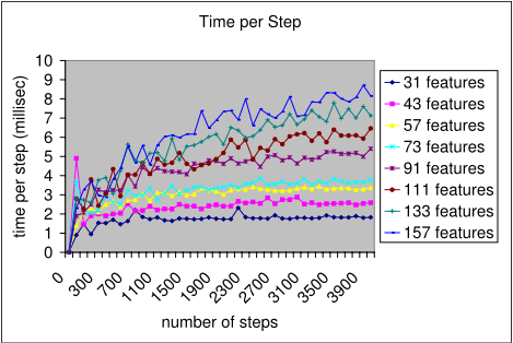
We tested our AE-STRIPS-SLAF algorithm in partially observable blocks-world domains. We generated random action-observation sequences of 4000 steps from a description of the domain in PDDL. Our SLAF algorithm receives no domain information besides the sequence of actions and observations that is given by the generator.

We ran the algorithm with blocks-world domains of increasing sizes (31 to 157 features). We collected the time and space taken for each time step in the execution, starting with zero knowledge. The results are shown in Figure 4. Each of the graphs belongs to a different domain size. They show that the time per step approaches a (very small, order of < 9 milliseconds) limit as the execution proceeds. The time that is taken to perform SLAF of different domains grows linearly with domain size.

Also, [Hlubocky and Amir, 2005] has included a modified version of this algorithm in their architecture and tested it on a suite of adventure-game-like virtual environments that are generated at random. These include arbitrary numbers of places, objects of various kinds, and configurations and settings of those. There, an agent's task is to exit a house, starting with no knowledge about the state space, available actions and their effects, or characteristics of objects. Their experiments show that the agent learns the effects of its actions very efficiently. This agent makes decisions using the learned knowledge, and inference with the resulting representation is fast (a fraction of a second per SAT problem in domains including more than 30 object, modes, and locations).

7 Comparison with RelatedWork

HMMs [Boyen and Koller, 1999; Boyen et al., 1999; Murphy, 2002; Ghahramani, 2001] can be used to estimate a stochastic transition model from observations. Unfortunately, HMMs require an explicit representation of the state space, and our smallest domain (31 features) requires a transition matrix of (231 )2 entries. This prevents initializing HMMs procedures on any current computer.

Structure learning approaches in Dynamic Bayes Nets (DBNs and also fHMMs) use EM and additional approximations (e.g., using factoring, variation, or sampling), and are more tractable. However, they are still limited to small domains (e.g., 10 features [Ghahramani and Jordan, 1997; Boyen et al., 1999]), and also have unbounded errors in discrete deterministic domains, so are not usable in our settings.

Reinforcement Learning (RL) approaches compute a mapping between world states and preferred actions. They are highly intractable in partially observable domains [Kaelbling et al., 1998], and approximation (e.g., [Kearns et al., 2000] is practical only for small domains (e.g., 10-20 features) with small horizon time T .

In contrast to HMMs, DBNs, and RL, our algorithms are exact and tractable in large domains (> 300 features). We take advantages of properties common to discrete domains, such as determinism, limited effects of actions, and observed failure.

Previous work on learning action models assumes fully observable deterministic domains. These learn parametrized STRIPS actions using, e.g., version spaces [Gil, 1994; Wang, 1995], general classifiers [Oates and Cohen, 1996], or hill-climbing ILP [Benson, 1995]. Recently, [Pasula et al., 2004] gave an algorithm that learns stochastic actions with no conditional effects. [Schmill et al., 2000] approximates partial observability by assuming that the world is fully observable. We can apply these to partially observable learning problems (sometimes) by using the space of belief states instead of world states, but this increases the problem size to exponentially, so this is not practical for our problem.

8 Conclusions

We presented a framework for learning the effects and preconditions of deterministic actions, and showed that in several common situations this can be done exactly in time that is polynomial (sometime linear) in the number of time steps and features. We can add bias and compute an exact solution for large domains (hundreds of features), in many cases.

The results that we presented are promising for many applications, including reinforcement learning, agents in virtual domains, and HMMs. Already, this work is being applied to autonomous agents in adventure games, and exploration is guided by the transition belief state that we compute and information gain criteria. In the future we plan to extend these results to stochastic domains, and domains with continuous features.

9 Acknowledgements

I wish to thank Megan Nance for providing the code and samples for the generator. I also wish to acknowledge support from DAF Air Force Research Laboratory Award FA8750-04-2-0222 (DARPA REAL program).