
Efficient Consequence Finding
Proceedings of the Seventeenth International Joint Conference on Artificial Intelligence. Pages 359-369.
© 2001 International Joint Conferences on Artificial Intelligence
Abstract
We present an extensive experimental study of consequence-finding algorithms based on kernel resolution, using both a trie-based and a novel ZBDD-based implementation, which uses ZeroSuppressed Binary Decision Diagrams to concisely store and process very large clause sets. Our study considers both the full prime implicate task and applications of consequence-finding for restricted target languages in abduction, model-based and faulttree diagnosis, and polynomially-bounded knowledge compilation. We show that the ZBDD implementation can push consequence-finding to a new limit, solving problems which generate over 1070 clauses.
- Bryant, 1992
- R. E. Bryant. Symbolic Boolean manipula- tion with ordered binary-decision diagrams. ACM Com- puting Surveys, 24(3):293-318, 1992.
- [Cadoli and Donini, 1997] M. Cadoli and F. M. Donini. A survey on knowledge compilation. AI Communications, 10:137-150, 1997.
- [Chandra and Markowsky, 1978] A. K. Chandra and G. Markowsky. On the number of prime implicants. Discrete Mathematics, 24:7-11, 1978.
- [Chatalic and Simon, 2000a] Ph. Chatalic and L. Simon. Davis and Putnam 40 years later: a first experimentation. Technical report, LRI, Orsay, France, 2000.
- [Chatalic and Simon, 2000b] Ph. Chatalic and L. Simon. Multi-resolution on compressed sets of clauses. In Proc. ICTAI (Tools with AI), pp. 449-454, 2000.
- [Chatalic and Simon, 2000c] Ph. Chatalic and L. Simon. Zres: The old Davis-Putnam procedure meets ZBDD. In CADE'00, Int. Conf. Automated Deduction, pp. 2-10, 2000.
- [Davis and Putnam, 1960] M. Davis and H. Putnam. A com- puting procedure for quantification theory. Journal of the ACM, 7(3):201-215, 1960.
- [de Kleer et al., 1992] J. de Kleer, A. K. Mackworth, and R. Reiter. Characterizing diagnosis and systems. Artificial Intelligence, 56:197-222, 1992.
- [de Kleer, 1986] J. de Kleer. An assumption-based TMS. Ar- tificial Intelligence, 28(2):127-162, 1986.
- [de Kleer, 1992] J. de Kleer. An improved incremental algo- rithm for generating prime implicates. In AAAI'92, Proc. 10th Nat. Conf. on Artificial Intelligence, pp. 780-785, 1992.
- [Dechter and Rish, 1994] R. Dechter and I. Rish. Direction- al resolution: The Davis-Putnam procedure, revisited. In KR'94, Proc. 4th Int. Conf. on Knowledge Representation and Reasoning, pp. 134-145.
- Morgan Kaufmann, 1994.
- A. del Val. An analysis of approximate knowledge compilation. In IJCAI'95, Proc. 14th Int. Joint Conf. on Artificial Intelligence, pp. 830-836, 1995. IJCAI
- A. del Val. A new method for conse- quence finding and compilation in restricted languages. In AAAI'99, 16th Nat. Conf. on Artificial Intelligence, p- p. 259-264, 1999.
- [del Val, 2000a] A. del Val. The complexity of restricted consequence finding and abduction. In AAAI'2000, Proc. 17th Nat. Conf. on Artificial Intelligence, pp. 337-342, 2000.
- [del Val, 2000b] A. del Val. Tractable classes for directional resolution. In AAAI'2000, Proc. 17th Nat. Conf. on Artifi- cial Intelligence, pp. 343-348, 2000.
- [Dimacs, 1992] The Dimacs challenge bench- marks. Originally available at ft- p://ftp.rutgers.dimacs.edu/challenges/sat. Link
- [El Fattah and Dechter, 1995] Y. El Fattah and R. Dechter. Diagnosing tree-decomposable circuits. In IJCAI'95, Proc. 14th Int. Joint Conf. on Artificial Intelligence, pp. 1742-1748, 1995. IJCAI
- [Inoue, 1992] K. Inoue. Linear resolution for consequence- finding. Artificial Intelligence, 56:301-353, 1992.
- [Kean and Tsiknis, 1990] A. Kean and G. Tsiknis. An incre- mental method for generating prime implicants/implicates. Journal of Symbolic Computation, 9:185-206, 1990.
- [Kean and Tsiknis, 1993] A. Kean and G. Tsiknis. Clause management systems. Computational Intelligence, 9:11- 40, 1993.
- [Marquis, 1999] P. Marquis. Consequence-finding algo- rithms. In D. Gabbay and Ph. Smets, editors, Handbook of Defeasible Reasoning and Uncertainty Managemen- t Systems (vol. 5): Algorithms for Defeasible and Uncer- tain Reasoning, pp. 41-145. Kluwer Academic Publishers, 1999.
- [Mathieu, 1991] Ph. Mathieu. L'utilisation de la logique trivaluée dans les systèmes experts. PhD thesis, Univer- sité des Sciences et Technologies de Lille, France, 1991.
- [Minato, 1993] S. Minato. Zero-suppressed BDDs for set manipulation in combinatorial problems. In Proc. 30th ACM/IEEE Design Automation Conf., pp. 272-277, 1993.
- [Prendinger et al., 2000] H. Prendinger, M. Ishizuka, and T. Yamamoto. The Hyper system: Knowledge reformation for efficient first-order hypothetical reasoning. In PRI- CAI'00, 6th Pacific Rim Int. Conf. on Artificial Intelli- gence, 2000.
- [Rauzy, 1996] A. Rauzy. Boolean models for reliability anal- ysis: a benchmark. Tech. report, LaBRI, Univ. Bordeaux I.
- [Reiter and de Kleer, 1987] R. Reiter and J. de Kleer. Foun- dations of assumption-based truth maintenance systems. In AAAI'87, 6th Nat. Conf. on Artificial Intelligence, 1987.
- [Schrag and Crawford, 1996] R. Schrag and J. Crawford. Implicates and prime implicates in random 3-SAT. Ar- tificial Intelligence, 81:199-221, 1996.
- [Selman and Kautz, 1996] B. Selman and H. Kautz. Knowl- edge compilation and theory approximation. Journal of the ACM, 43(2):193-224, 1996.
- [Selman and Levesque, 1996] B. Selman and H. J. Levesque. Support set selection for abductive and default reasoning. Artificial Intelligence, 82:259-272, 1996.
- [Tison, 1967] P. Tison. Generalized consensus theory and application to the minimization of boolean circuits. IEEE Transactions on Computers, EC-16:446-456, 1967.
References were extracted automatically from the PDF and may contain errors.
Full text extracted automatically from the PDF; figures, tables and equations may differ. The PDF is the version of record.
1 Introduction
Many tasks in Artificial Intelligence can be posed as consequence-finding tasks, i.e. as the problem of finding certain consequences of a propositional knowledge base. These include prime implicates, abduction, diagnosis, nonmonotonic reasoning, and knowledge compilation. [Marquis, 1999] provides an excellent survey of the field and its applications. Unfortunately, there have been very few serious computational attempts to address these problems. After some initial excitement with ATMSs [de Kleer, 1986] and clause management systems [Reiter and de Kleer, 1987; Kean and Tsiknis, 1993], it was soon realized that these systems would often run out of resources even on moderately sized instances, and interest on the topic waned. Thus, for example, [Marquis, 1999] says in concluding his survey:
"The proposed approaches [to consequencefinding] are however of limited computational scope (algorithms do not scale up well), and there is only little hope that significantly better algorithms could be designed"
In this paper, we conduct the first extensive experimental study of consequence-finding (CF), more specifically of one of the approaches referred to in the above quote, namely kernel resolution [del Val, 1999]. Kernel resolution allows very efficient focusing of consequence-finding on a subset of "interesting" clauses, similar to SOL resolution [Inoue,
Alvaro del Val
E.T.S. Inform´atica, B-336 Universidad Aut ´onoma de Madrid 28049 Madrid, Spain delval@ii.uam.es
1992]. We also introduce novel consequence-finding technology, namely, the use of ZBDDs (Zero-Suppressed Binary Decision Diagrams [Minato, 1993]) to compactly encode and process extremely large clause sets. As a result of this new technology, the well-known Tison method [Tison, 1967] for finding the prime implicates of a clausal theory, a special case of kernel resolution, can now efficiently handle more than 1070 clauses. The combination of focused consequencefinding with ZBDDs makes CF able to deal computationally with significant instances of the applications discussed above for the first time. In particular, our experiments include both full CF (the prime implicate task), and applications of consequence-finding for restricted target languages in abduction, model-based and fault-tree diagnosis, and polynomiallybounded knowledge compilation.
We assume familiarity with the standard literature on propositional reasoning and resolution. Some definitions are as follows. A clause C subsumes a clause D iff C ⊆ D. The empty clause is denoted ✷. For a theory (set of clauses) Σ, we use µ(Σ) to denote the result of removing all subsumed clauses from Σ. An implicate of Σ is a clause C such that Σ |= C; a prime implicate is an implicate not subsumed by any other implicate. We denote by PI(Σ) the set of prime implicates of Σ. We are often interested only in some subset of PI(Σ). For this purpose, we define the notion of a target language LT , which is simply a set of clauses. We assume LT is closed under subsumption (c.u.s.), i.e. for any C ∈ LT and D ⊆ C, we have D ∈ LT . A target language can always be closed under subsumption by adding all subsumers of clauses in the language.
Given these definitions, the task we are interested in is finding the prime LT -implicates of Σ, defined as PILT (Σ) = PI(Σ) ∩ LT . We will mainly consider the following target languages: L is the full language, i.e. the set of all clauses over the set V ar(Σ) of variables of Σ. L✷ = {✷} contains only the empty clause. Given a set of variables V , the "vocabulary-based" language LV is the set of clauses over V . Finally, for a constant K, LK is the set of clauses over V ar(Σ) whose length does not exceed K. Thus we have L1, L2, etc.
Each of these languages corresponds to some important AI task. At one extreme, finding the prime implicates of Σ is simply finding PIL(Σ) = PI(Σ); at the other extreme, deciding whether Σ is satisfiable is identical to deciding whether PIL✷ (Σ) is empty. Vocabulary-based languages also have many applications, in particular in abduction, diagnosis, and non-monotonic reasoning (see e.g. [Inoue, 1992; Selman and Levesque, 1996; Marquis, 1999] among many others). Finally, LK or subsets thereof guarantee that PILK (Σ) has polynomial size, which is relevant to knowledge compilation (surveyed in [Cadoli and Donini, 1997]).
Sometimes we will be interested in theories which are logically equivalent to PILT (Σ), but which need not include all LT -implicates, and can thus be much more concise. We refer to any such theory as a LT -LUB of Σ, following [Selman and Kautz, 1996], see also [del Val, 1995]. We'll see one particular application of LT -LUBs in our discussion of diagnosis later.
2 Kernel resolution: Review
Kernel resolution, described in [del Val, 1999; 2000a], is a consequence-finding generalization of ordered resolution. We assume a total order of the propositional variables x1, . . . , xn. A kernel clause C is a clause partitioned into two parts, the skip s(C), and the kernel k(C). Given any target language LT closed under subsumption, a LT -kernel resolution deduction is any resolution deduction constructed as follows: (a) for any input clause C, we set k(C) = C and s(C) = ∅; (b) resolutions are only permitted upon kernel literals; (c) the literal l resolved upon partitions the literals of the resolvent into those smaller (the skip), and those larger (the kernel) than l, according to the given ordering; and (d) to achieve focusing, we require any resolvent R to be LT - acceptable, which means that s(R) ∈ LT .
In order to search the space of kernel resolution proofs, we associate to each variable xi a bucket b[xi] of clauses containing xi. The clauses in each bucket are determined by an indexing function ILT , so that C ∈ b[xi] iff xi ∈ ILT (C). We can always define ILT (C) = {kernel variables of the largest prefix l1 . . . lk of C s.t. l1l2 . . . lk-1 ∈ LT}, where C is assumed sorted in ascending order [del Val, 1999]; resolving on any other kernel literal would yield a non-LT -acceptable resolvent.
Bucket elimination, abbreviated LT -BE, is an exhaustive search strategy for kernel resolution. LT -BE processes buckets b[x1], . . . , b[xn] in order, computing in step i all resolvents that can be obtained by resolving clauses of b[xi] upon xi, and adding them to their corresponding buckets, using ILT . We denote the set of clauses computed by the algorithm as LT -BE(Σ). The algorithm, which uses standard subsumption policies (so that LT -BE(Σ) = µ(LT -BE(Σ))), is complete for finding consequences of the input theory which belong to the target language LT , that is, LT -BE(Σ)∩LT = PILT (Σ).
As shown in [del Val, 1999], L-BE is identical to Tison's prime implicate algorithm [Tison, 1967], whereas L✷-BE is identical to directional resolution (DR), the name given by [Dechter and Rish, 1994] to the original, resolution-based Davis-Putnam satisfiability algorithm [Davis and Putnam, 1960]. L✷-BE(Σ) is called the directional extension of Σ, and denoted DR(Σ).
For LV we will in fact consider two BE procedures, both of which assume that the variables of V are last in the order- BDD
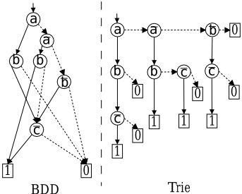
Figure 1: ZBDD and trie representation for the set of clauses Σ = {a ∨ b ∨ ¬c, ¬a ∨ b, ¬a ∨ ¬c, ¬b ∨ ¬c}.
ing. L1V -BE is simply LV -BE under this ordering assumption. L0V -BE is identical, except that processing is interrupted right before the first variable of V is processed. Thus L1V -BE(Σ) ∩ LV = PILV (Σ), whereas L0V -BE(Σ) ∩LV is logically equivalent but not necessarily identical to PILV (Σ); i.e., it is a LV -LUB of Σ. Note that, in either case, the desired set of clauses is stored in the last buckets. The advantage of this ordering is that either form of LV -BE behave exactly as directional resolution, a relatively efficient satisfiability method, up to the first V -variable of the ordering. L0V -BE stops right there (and is thus strictly cheaper than deciding satisfiability with DR under such orderings), while L1V -BE continues, computing the prime implicates of L0V -BE(Σ) ∩ LV with full kernel resolution over the V - buckets.
3 Zero-Suppressed BBDs: Review
[Bryant, 1992] provides an excellent survey and introduction of Binary Decision Diagrams (BDD). A BDD is a directed acyclic graph with a unique source node, only two sinks nodes (1 and 0, interpreted respectively as true and false) and with labeled nodes ∆(x, n1, n2). Such node x has only two children (n1 and n2, connected respectively to its 1arc and 0-arc) and is classically interpreted as the function f = if x then f1 else f2 (if f1 and f2 interpret the BDDs n1 and n2).
The power of BDDs derives from their reduction rules. A ROBDD (Reduced Ordered BDD, simply noted BDD in the following) requires that its variables are sorted according to a given order and that the graph does not contain any isomorphic subgraph (node-sharing rule). In addition, the nodeelimination rule deletes all nodes ∆(x, n, n) that do not care about their values. With the classical semantics, each node is labeled by a variable and each path from the source node to the 1-sink represents a model of the encoded formula. The BDD can thus be viewed as an efficient representation of a Shannon normal tree.
In order to use the compression power of BDDs for encoding sparse sets instead of just boolean functions, [Minato, 1993] introduced Zero-Suppressed BDDs (ZBDDs). Their principle is to encode the boolean characteristic function of a set. For this purpose, Minato changed the node-elimination rule into the Z-elimination rule for which useless nodes are those of the form ∆(x, 0, n). So, if a variable does not appear on a path, then its default interpretation is now false (which means absent, instead of don't care). If one wants to encode only sets of clauses, each ZBDD variable needs to be labeled by a literal of the initial formula, and each path to the 1-sink now represents the clause which contains only the litterals labeling the parents of all 1-arcs of this path. Figure 1 represents the ZBDD encoding the set of clauses Σ = {a ∨ b ∨ ¬c, ¬a ∨ b, ¬a ∨ ¬c, ¬b ∨ ¬c}.
The "compressing" power of ZBDDs is illustrated by the fact that there exist theories with an exponential number of clauses that can be captured by ZBDDs of polynomial size. Because their complexity only depends on the size of the ZBDD, not on the size of the encoded set, ZBDD operators can be designed to efficiently handle sets of clauses of an exponential size.
4 Kernel resolution on ZBDDs
In order to deal with this compact encoding in the context of kernel resolution, we need to define a way to efficiently obtain resolvents, and to identify buckets. For the former task, [Chatalic and Simon, 2000b; 2000c] introduced a very efficient multiresolution rule which works directly on sets of clauses, and thus which can compute the result of eliminating a variable without pairwise resolving clauses.
Definition (multiresolution): Let ∆+ and ∆- be two sets of clauses without the variable xi. Let Ri be the set of clauses obtained by distributing the set ∆+ over ∆-. Multiresolution is the following rule of inference:
A bucket b[xi] can always be expressed in the form required by this rule, so that Ri corresponds to the set of resolvents obtained by processing b[xi]. The main advantage of this definition is that it can be shown that if Ri is computed directly at the set level, without explicitly enumerating clauses, its complexity can be independent of the number of classical resolution steps. [Chatalic and Simon, 2000b] propose a system called ZRes which implements the multiresolution principle by means of ZBDDs. ZRes manipulates clause sets directly, through their ZBDD representation, with no explicit representation of individual clauses. A bucket is easily retrieved from the ZBDD storing the current clause set in the form of ZBDDs for appropriate ∆+i and ∆-i ; and it is then processed using a specialized ZBDD operator, clausedistribution, which implements multiresolution by distributing ∆+i over ∆-i to obtain Ri. The system comes with other ZBDDs operators designed for clause-set manipulation, such as subsumption-free union and set-difference. All these three operators delete subsumed and tautologous clauses as soon as possible, during the bottom-up construction of the resulting ZBDD.
To generalize these ideas for focused kernel resolution, we need to deal with complex indexing functions. For this purpose, we keep two ZBDDs, for dead and live clauses respectively. A "dead" clause is one which can no longer be resolved according to the LT -restriction in place, given the variables that have been processed so far. For example, a clause becomes dead for L✷ (i.e. for DR) when just one of its variables is processed; and for LK when its first K + 1 variables are processed. Right before processing a variable, we obtain "its bucket" from the live ZBDD. Processing the variable is then done by multiresolution. Finally, when done with a variable, new clauses become dead, and they are moved from the live ZBDD to the dead ZBDD.
5 Experimental results
Our experimental tests, which include structured benchmark gathering and generating as well as random instances testing, represents more than 60 cpu-days on the reference machine 1 , more than 10000 runs on structured examples and almost the same on random instances. Only selected results are presented here, for an obvious lack of space.
Times are reported in seconds. All experiments use a 1000 seconds timeout, and a dynamic min-diversity heuristic for variable ordering. This heuristic chooses the variable for which the product of its numbers of positive and negative occurrences is minimal, thus trying to minimize the number of resolvents.
In addition to the ZBDD-based implementations, labeled zres, we also consider algorithms based on the trie-data structure [de Kleer, 1992], namely, picomp and drcomp, for respectively prime implicates and directional resolution. In contrast to the ZBDD programs, trie-based programs explicitly represent clauses and buckets, and use pairwise resolution. The trie (illustrated in Figure 1) includes a number of significant optimizations to minimize trie traversal, for efficient subsumption.
It can be shown that ZBDDs are never worse than tries in space requirements, and can be much better. Intuitively, while tries can only share common structure on the prefix of clauses, ZBDDs can do it on their prefix and postfix, i.e. they allow factoring clauses from both the beginning and the end. In terms of time, as we will see, the situation is more complex. Nevertheless, the ZBDD implementation is the one that really pushes consequence-finding well beyond its current limits.
5.1 Prime implicates
Prime implicate computation remains one of the fundamental consequence finding tasks. We focus in this section on our two very different Tison's algorithm implementations, picomp and zres-tison. We use the following benchmarks, among others: chandra-n [Chandra and Markowsky, 1978] and mxky [Kean and Tsiknis, 1990] are problems with known exponential behavior; adder-n (n-bit adders), serial-adder (n-bit adders obtained by connecting n full adders), bnp-n-p (tree-structured circuits with n layers, where p is a probability, [El Fattah and Dechter, 1995]) represent digital circuits; serial-diag-adder and bnp-ab represent the same circuits in a form suitable for diagnostic reasoning; pipes and pipes-syn are problems drawn from qualitative physics; type-k-n problems, due to [Mathieu, 1991], attempt to mimic "typical" structures of expert system KBs, with each k representing a particular kind of structure.
1 On the Dimacs [Dimacs, 1992] machine scale benchmark, this Pentium-II 400MHz has a time saving of 305%
| Benchmark | #PIs | picomp | zres-tison |
|---|---|---|---|
| adder-10 | 826457 | 171 | 1.07 |
| adder-50 | 1.0e+25 | - | 172 |
| adder-100 | 7.2e+48 | - | 381 |
| chandra-21 | 2685 | 0.1 | 0.29 |
| chandra-100 | 9.2e+15 | - | 12.23 |
| chandra-400 | 2.8e+63 | - | 318 |
| bnp-5-50-ts4-rr-2 | 1240 | 0.02 | 0.42 |
| bnp-7-50-ts4-rr-1 | 5.7e+6 | - | 10.9 |
| bnp-7-50-ts4-rr-2 | 3.0e+10 | - | 15.9 |
| bnp-ab-5-50-ts4-rr-2 | 1641 | 0.04 | 0.80 |
| bnp-ab-7-50-ts4-rr-2 | 7.2e+10 | - | 311 |
| m6k6 | 823585 | 1.18 | 0.36 |
| m9k8 | 1.0e+8 | - | 1.81 |
| m30k25 | 1.9e+37 | - | 256 |
| n-queens-5 | 3845 | 1.72 | 4.26 |
| pigeons-5-5 | 7710 | 12.4 | 49.6 |
| pigeons-6-5 | 17085 | 93.5 | 356 |
| pipes-simple-08 | 71900 | 390 | 38.9 |
| pipes-simple-12 | 321368 | - | 239 |
| pipes-syn-10 | 30848 | 35.2 | 2.69 |
| pipes-syn-40 | 4.3e+6 | - | 518 |
| serial-adder-10-4 | 8.4e+7 | - | 4.33 |
| serial-adder-30-4 | 6.4a+21 | - | 717 |
| serial-diag-adder-10-4 | 1.7e+10 | - | 78.3 |
| serial-diag2-8-0b | 2.2e+8 | - | 11.7 |
| type1-800 | 319600 | 16.4 | 219 |
| type5-150 | 3.7e+71 | - | 330 |
The first observation that can be drawn from Table 1 is the scalability of zres-tison, which can handle a huge number of clauses on some particular instances (e.g. 1071 for type5-150). Thus it forces us to completely reconsider Tison's algorithm efficiency and limitations. In all these examples, picomp simply cannot physically represent such sets of clauses and, like all previous Tison's implementations, is no competition for zres-tison. Yet, on some instances, picomp remains faster. This is due to small distributions computation, involving less than a thousand clauses (e.g. type-1-800) at each multiresolution step. On such examples, traditional approaches with explicit representation of clauses remain faster. Notice finally the relative independence of the running time of zres-tison w.r.t. the number of PIs, in contrast to picomp. For zres-tison there are easy examples with a huge number of PIs, and hard examples with few PIs. The latter include n-queens and satisfiable pigeon problems, which contrasts with the excellent results for satisfiability of similar problems in [Chatalic and Simon, 2000c].
5.2 Polynomial size compilation
One of the major theoretical limits of knowledge compilation (KC) is that it is very unlikely that a KC method can be defined that always produces tractable compiled theories of polynomial size, unless we restrict the query language to have polynomial size. That's what LK-BE does. To implement this with zres, clauses having more than k processed variables are moved to the dead ZBDD. We test here only the zres-kbound implementation with different k on the same benchmarks used on prime implicates. Summarizing so many test runs on so many different benchmarks families is not easy. We attempt to do so in Table 2, where a cell on row i and column j contains the percentage of benchmarks quickly solved by the program i in comparison with program j. For instance, zres-kbound(3) terminates more quickly than zres-tison in 31% of the cases, and the median value of the cpu gain is 3.70. Of course, such a table can't take into account the particularities of each benchmark family, but it still can give some taste of how the different approaches behave with respect to each other.
| k(3) | k(4) | k(5) | k(6) | z-tison | |
|---|---|---|---|---|---|
| k(3) | - | 52 (1.19) | 46 (1.45) | 46 (1.45) | 31 (3.70) |
| k(4) | 31 (1.04) | - | 41 (1.18) | 41 (1.18) | 23 (2.75) |
| k(5) | 37 (1.05) | 35 (1.06) | - | 0 | 18 (2.21) |
| k(6) | 37 (1.05) | 35 (1.06) | 0 | - | 18 (2.21) |
| z-tison | 53 (2.88) | 56 (2.83) | 58 (2.88) | 58 (2.88) | - |
What is striking is that Tison remains the fastest procedure in most cases, with a median cpu gain of around 285%. But, we can see that, in 31% of the cases, kbound(3) performmuch better than zres-tison. This phenomenon (also observed with kbound(4-6)) means that when zres-tison fails, kbound remains an available solution. Moreover, our results suggest that kbound(5) and kbound(6) perform similarly, yet the latter computes a much more interesting base.
5.3 Directional resolution
Directional resolution compiles a theory into an equivalent one in which one can generate any model in linear time. We test here our two DR implementations, drcomp and zres, on some specific benchmarks, with two heuristics for each one. In Table 3 the par-8-*, pret150-25, ssa0432 files are taken from the Dimacs database, and #KB means the size of the theory obtained by the programs. As this size depends on the order of variable deletions, we only report it for the first case, where the two programs give the same result.
As shown in Table 3, good heuristics have a major effect. Using just input ordering often forces the size of the KB to grow in such a way that drcomp can't compete with zres. ZBDDs pay off in all these cases, showing their ability to represent very large KBs. The min-diversity heuristics seems to invert the picture, mainly because the ordering helps to keep the clause set to manageable size (tens of thousands of clauses). The same applies to theories which are tractable for directional resolution, such as circuit encodings [del Val, 2000b], for which drcomp takes no time. zres, in contrast, seems to include a significant overhead on theories which do not generate many clauses, despite its relatively good performance reported in [Chatalic and Simon, 2000b]. On the other hand, ZBDDs scale much better when dealing with very large KBs.
| Input Order | Min Diversity | ||||
|---|---|---|---|---|---|
| Bench. | #KB | zres | drcomp | zres | drcomp |
| adder-400 | 7192 | 482 | 1.36 | 310 | 1.23 |
| chandra-400 | 1.3e+36 | 132 | - | 28.2 | 0.02 |
| m8k7 | 2396801 | 1.19 | 24.05 | 0.50 | 0.01 |
| m30k25 | 8.76e+37 | 292 | - | 79.1 | 0.05 |
| par8-2-c | 15001 | 332 | - | 1.24 | 0.04 |
| par8-2 | 350 | - | 476.82 | 30.31 | 0.10 |
| pret150-25 | 1.75e+15 | 8.69 | - | 4.83 | 20.8 |
| ssa0432-003 | 2.01e+9 | 407 | - | 45.2 | 0.01 |
| type1-850 | 849 | 99.9 | 0.08 | 91.5 | 0.11 |
5.4 Abduction
Given a theory Σ and a set A of variables (called assumptions, hypothesis or abducibles), an abductive explanation of a clause C wrt. Σ is a conjunction L of literals over A such that Σ ∪ L is consistent and entails C (or a subsumed clause of C). L is a minimal explanation iff no subset of it is also an explanation.
On the adder-n, mult-n (adder and multiplier whose result is smaller than n), and on the bnp circuits introduced in section 5.1, we are given a circuit Σ with a set of input variables I and output variables O. We want to explain some observation (an instantiation of some O variables) with only variables from I (thus forgetting all internal variables). This problem can be addressed through LV -BE with V = I ∪ O. In this case, the trie-based implementation failed in all benchmarks (except adder-5), so we only report results for the ZBDD-based implementation, in Table 4. We also tried our algorithms on the ISCAS circuits benchmark family, without success. To interpret these results appropriately, one should note that obtaining PILV means precomputing answers for all abduction problems for Σ, as explanations can be directly read off from PILV (Σ). Kernel resolution also provides methods for answering only specific abduction problems (as opposed to all), but we have not tested them; for some tests with a similar flavor, check the diagnosis experiments on ISCAS benchmarks, section 5.6.
Note that, surprisingly, all adder examples are treated much more efficiently by zres-tison (table 1) than by L1V -BE. A similar phenomenon was already pointed out in [Chatalic and Simon, 2000a], where, on some examples, computing DR on a subset of variables was proved harder than on the whole set of variables (L0V -BE harder than L0A-BE, where V ⊆ A). But, here, in addition, the induced hardness overcomes the simplification due to the use of DR instead of Tison, which is clearly counter-intuitive. This is not the case for the mult-n nor for the bnp-10-50 instances, on which picomp and zres-tison failed.
Table 5 presents some easier examples, the path-kr problems from [Prendinger et al., 2000] (abbreviated p-kr), which can be solved by both drcomp and picomp. For comparison with their results, note that we, unlike them, are solving all abduction problems for the given instance in one go.
| L0V | L1V | |||
|---|---|---|---|---|
| Bench. | Time | #LV -LUB | Time | #P ILV |
| adder-5 | 0.18 | 448 | 0.3 | 1396 |
| adder-10 | 0.78 | 18184 | 3.6 | 354172 |
| adder-20 | 3.51 | 1.88e+7 | 36.51 | 2.09e+10 |
| adder-25 | 5.88 | 6.03e+8 | - | - |
| adder-100 | 423.51 | 2.28e+32 | - | - |
| mult-16 | 0.66 | 275 | 4.47 | 1918 |
| mult-64 | 16.86 | 3466 | - | - |
| mult-128 | 2.25 | 1307 | 585.99 | 39398 |
| bnp-7-50-1 | 6.12 | 193605 | 6.39 | 193605 |
| bnp-7-50-3 | 5.97 | 24435 | 6.33 | 24435 |
| bnp-10-50-3 | 805.53 | 2.30e+14 | - | - |
| bnp-10-50-4 | 671.61 | 1.76e+19 | - | - |
| Bench. | #KB | zres | drcomp | #PIs | zres-tis. | picomp |
|---|---|---|---|---|---|---|
| p-2r | 28 | 0.24 | 0.03 | 80 | 0.30 | 0.03 |
| p-6r | 7596 | 31.3 | 0.33 | 1332 | 48.5 | 0.36 |
| p-10r | 99100 | 374 | 18.7 | 122000 | 360 | 22.9 |
5.5 Fault-Tree Diagnosis
The set of Aralia [Rauzy, 1996] benchmarks arise from fault tree diagnosis, in which one wants to characterize the set of elementary failures (coded by the fi predicates) that entail the failure of the whole system (the root predicate). It thus amounts to computing the set of LV -implicants of the root, where V is the set of fi. We use the well-known duality cnf/dnf and implicants/implicates to express those problems as LV -implicates problems.
Usually, these benchmarks are efficiently solved using traditional BDDs approaches (i.e. rewritting the initial formula under Shannon Normal Form). In [Rauzy, 1996], internal variables (defined as an equivalency with a subformula), are not even encoded in the BDD: they are directly identified with the BDD encoding the subformula. In our approach, such internal variable are explicitly present in the cnf of the formula. The work of zres amounts to precisely delete all of them, thus obtaining a formula build on fi (and the root) predicates. In table 6, we show that kernel resolution, with multiresolution, can efficiently handle those problems without needing to rewrite the formula under Shannon Normal Form. To our knowledge, this is the first time that such direct CF approach successes.
5.6 Model-based diagnosis
In diagnosis [de Kleer et al., 1992], we are given a theory Σ describing the normal behavior of a set of components; for each component, there is an "abnormality" predicate abi. Let V = AB be the set of abi's. Given a set of observations O, the diagnosis are given by the prime LV -implicants (noted PALV ) of PILV (Σ ∪ O). As we can obtain these implicants from any equivalent LV -LUB of Σ, either L1V -BE or L0V -BE can yield the diagnosis, so we use the cheaper L0V -BE.
| Benchmark | zres | #PILV |
| baobab2 | 1.9 | 1259 |
| baobab3 | 16.32 | 24386 |
| das9205 | 0.61 | 17280 |
| das9209 | 11.98 | 8.2e+10 |
| edf9205 | 15.4 | 21308 |
| edf9206 | 669.3 | 7.15e+9 |
| isp9602 | 17.05 | 5.2e+7 |
| isp9605 | 1.67 | 1454 |
| Bench. | T. L0V -BE | #LV -LUB | T. PALV | #PALV |
|---|---|---|---|---|
| c432-d-03 | 99.16 | 1648704 | 315.13 | 1243 |
| c432-d-06 | 462.16 | 3549876 | - | - |
| c432-d-09 | 140.60 | 18084 | 180.67 | 6651166 |
| c499-d-03 | 42.14 | 102 | 470.12 | 7347194 |
| c499-d-04 | 43.39 | 227 | - | - |
| c499-d-09 | 68.51 | 1065 | 198.74 | 3.2e+7 |
| c880-d-03 | 98.16 | 174 | 103.13 | 13349 |
| c880-d-08 | 98.96 | 87 | 99.65 | 698 |
| c880-d-05 | 153.35 | 1 | 153.47 | 23 |
| c1355-d-01 | 268.48 | 965 | - | - |
| c1355-d-02 | 233.46 | 182 | - | - |
| c1355-d-10 | 224.89 | 11 | 225.57 | 49856 |
We first consider ISCAS benchmarks. We generated for each of the four easiest circuits their normal behavior formula (by introducing abi variables on each gate), and 10 faulty input-output vectors. The results are given in Table 7 (with T. denoting the total time), only for the ZBDD-based implementation. In a number of cases (where LV -LUB is of reasonable size), drcomp can also go through the first phase, but our current implementation fails to complete the second phase, thus we don't report its results here. To generate the implicants with our ZBDD-based system, we use one of its procedures that can negate a given formula. 3 of the 40 instances were too hard for L0V -BE, and 14 failed to compute the LV -implicants. To our knowledge, this is the first time such instances are tested with a direct consequence-finding approach.
Table 8 presents results for bnp-ab circuits for the much harder "compiled" approach to diagnosis, where we basically precompute PILV for all possible input-output vectors, by computing PILAB∪O∪I . Clearly, in this case it pays off to use the vocabulary-based procedures (as opposed to full PIs) for both tries and ZBDDs.
5.7 Random instances
Finally, we consider random instances generated with the fixed clause-length model. While conclusions drawn from them do not say anything about the behavior of algorithms on structured and specially real-world instances, they provide in our case a good tool for evaluating subsumption and optimization techniques for resolution. It was observed in
| Bench. | #KB | zres | drcomp | #PIs | zres-tis. | picomp |
|---|---|---|---|---|---|---|
| bnp-5-1 | 200 | 0.54 | 0.03 | 6441 | 0.90 | 0.24 |
| bnp-5-3 | 35 | 0.48 | 0.03 | 724 | 1.02 | 0.03 |
| bnp-7-1 | 78109 | 19.26 | 21.6 | 1.3e+8 | 30.4 | - |
| bnp-7-2 | 31166 | 8.55 | 52.1 | 1.7e+11 | 33.9 | - |
| bnp-7-4 | 110829 | 13.89 | - | 8.2e+8 | 32.8 | - |
| Program | Mean | Med. | Std | 50% int. | #Uns.(MT) |
|---|---|---|---|---|---|
| zres-tison | 8.15 | 3.43 | 14.03 | 1.32-8.95 | 0 (232) |
| picomp | 32.79 | 9.79 | 64.61 | 2.72-27.78 | 42 |
| zres-kbound 3 | 3.78 | 2.67 | 3.61 | 1.57-4.71 | 0 (34.3) |
| zres-kbound 4 | 7.48 | 3.93 | 10.28 | 1.83-8.66 | 0 (152) |
| zres-kbound 5 | 8.86 | 3.97 | 14.52 | 1.81-9.61 | 0 (218) |
[Dechter and Rish, 1994; Chatalic and Simon, 2000a] that such instances are very hard for DR, and [Schrag and Crawford, 1996] observed even worse behavior for consequencefinding for instances generated near the SAT phase transition threshold. Using a more powerful computer than in the previous benchmarks 2 , we compare picomp, zres-tison, and zres-kbound on 1000 formulae at the ratio 4 (30 variables, 120 clauses, 80% satisfiable). If we focus on satisfiable theories, their mean number of prime implicates is 494 (std: 1595; median: 65; 50% confidence interval: 30-254; max: 20000). Table 9 summarizes cpu-time results (the last column is the number of unsolved instances and the maximal cpu time needed if all instances have been solved).
We observe from this table that ZBDDs are always better than tries on random instances. For instance, with zrestison, the maximal number of clauses reached by each run has a median of 4890 (mean; 5913, std: 4239, 50% int: 2891-8022, max: 30147), but the maximal number of ZBDDs nodes has only a median of 3393 (mean: 3918, std: 2522, 50% int: 2096-5236, max: 19231). This gives less than one node per clause on average, despite the fact that most of the clauses are longer than 4. Even if such instances are "unstructured", at the beginning of the calculus, resolution (which we have seen really amounts to clause distribution) introduces many redundancies in formulae, which seem to be well-captured by ZBDDs.
6 Conclusion
We presented an extensive experimental study of consequence-finding, including results on many of its applications, using two quite different implementations. By combining the focusing power of kernel resolution with the ZBDD representation and multiresolution, we have shown the scalability of our approach and the relative independance of its performances with respect to the size of the handled KB. The until now mainly theoretical applications of CF can now be approached for problems of realistic size, and in some cases of spectacular size.
2 AMD-Athlon 1GHz running Linux with a Dimacs machine scale of 990% cpu savings.
@inproceedings{ijcai2001p51,
  title     = {Efficient Consequence Finding},
  author    = {Simon, Laurent and del Val, Alvaro},
  booktitle = {Proceedings of the Seventeenth International Joint Conference on
               Artificial Intelligence, {IJCAI-01}},
  publisher = {International Joint Conferences on Artificial Intelligence},
  editor    = {Bernhard Nebel},
  pages     = {359--369},
  year      = {2001},
  url       = {https://ijcai.org/proceedings/2001/51},
}
TY - CPAPER TI - Efficient Consequence Finding AU - Simon, Laurent AU - del Val, Alvaro T2 - Proceedings of the Seventeenth International Joint Conference on Artificial Intelligence, IJCAI-01 PB - International Joint Conferences on Artificial Intelligence PY - 2001 SP - 359 EP - 369 UR - https://ijcai.org/proceedings/2001/51 ER -Copied
Machine-readable versions of this paper, for tools and AI agents:





