
Ranking Cases with Decision Trees: a Geometric Method that Preserves Intelligibility
Proceedings of the Nineteenth International Joint Conference on Artificial Intelligence. Pages 635-639.
Abstract
This paper proposes a new method to rank the cases classified by a decision tree. The method applies a posteriori without modification of the tree and doesn’t use additional training cases. It consists in computing the distance of the cases to the decision boundary induced by the decision tree, and to rank them according to this geometric score. When the data are numeric it is very easy to implement and efficient. The distance-based score is a global assess, contrary to other methods that evaluate the score at the level of the leaf. The distance-based score gives good results even with pruned tree, so if the tree is intelligible this property is preserved with an improved ranking ability. The main reason for the efficacity of the geometric method is that in most cases when the classifier is sufficiently accurate, errors are located near the decision boundary.
- [Adams and Hand, 1999] N. M. Adams and D. J. Hand. Comparing classifiers when the misallocation costs are un- certain. Pattern Recognition, 32(7):1139-1147, 1999.
- [Alvarez, 2004] Isabelle Alvarez. Explaining the result of a decision tree to the end-user. In Proceedings of the 16th European Conference on Artificial Intelligence, pages 119-128, Valencia, Spain, Aout 2004.
- Morgan Kaufmann.
- [Blake and Merz, 1998] C.L. Blake and C.J. Merz. UCI repository of machine learning databases, 1998.
- [Bradley and Lovell, 1995] Andrew P. Bradley and Brian C. Lovell. Cost-sensitive decision tree pruning: Use of the roc curve. In Eighth Australian Joint Conference on Artificial Intelligence, pages 1-8, 1995.
- [Breiman et al., 1984] L. Breiman, J. H. Friedman, R. A. Ol- shen, and C. J. Stone. Classification and Regression Trees. Wadsworth, Belmont, 1984.
- [Cestnik, 1990] B. Cestnik. Estimating probabilities: A cru- cial task in machine learning. In Proceedings of the Euro- pean Conference on Artificial Intelligence, pages 147-149, 1990.
- [Esposito et al., 1997] F. Esposito, D. Malerba, and G. Se- meraro. A comparative analysis of methods for pruning decision trees. IEEE Transactions on Pattern Analysis and Machine Intelligence, 19(5):476-491, 1997.
- [Kohavi, 1996] Ron Kohavi. Scaling up the accuracy of naive-bayes classifiers: a decision-tree hybrid. In Proceed- ings of the Second International Conference on Knowl- edge Discovery and Data Mining, pages 202-207, 1996.
- [Ling and Yan, 2003] C. X. Ling and R. J. Yan. Decision tree with better ranking. In Proceedings of the 20th Interna- tional Conference on Machine Learning, pages 480-487, 2003.
- [Murthy, 1998] S.K. Murthy. A automatic construction of decision trees from data: A multi-disciplinary survey. Data Mining and Knowledge Discovery, 2(4):345-389, 1998.
- [Platt, 2000] J. Platt. Probabilistic outputs for support vec- tor machines. In Bartlett P. Schoelkopf B. Schuurmans D. Smola, A.J., editor, Advances in Large Margin Classi- fiers, pages 61-74, Cambridge, Massachusetts, 2000. MIT Press.
- [Provost and Domingos, 2003] F. Provost and P. Domingos. Tree induction for probability-based ranking. Machine Learning, 52(3):199-215, 2003.
- [Quinlan, 1993] J.R. Quinlan. C4.5: Programs for Machine Learning. Morgan Kaufmann, San Mateo, 1993.
- [Smyth et al., 1995] Padhraic Smyth, Alexander Gray, and Usama M. Fayyad. Retrofitting decision tree classifiers us- ing kernel density estimation. In International Conference on Machine Learning, pages 506-514, 1995.
- [Umano et al., 1994] M. Umano, K. Okomato, I. Hatono, H. Tamura, F. Kawachi, S. Umezu, and J. Kinoshita. Fuzzy decision trees by fuzzy id3 algorithm and its application to diagnosis systems. In 3rd IEEE International Conference on Fuzzy Systems, pages 2113-2118, 1994.
- [Witten and Frank, 2000] I. Witten and E. Frank. Data Min- ing: Practical Machine Learning Tools and Techniques with Java Implementation. Morgan Kaufmann, 2000.
- [Zadrozny and Elkan, 2001] Bianca Zadrozny and Charles Elkan. Obtaining calibrated probability estimates from de- cision trees and naive bayesian classifiers. In Proc. 18th International Conf. on Machine Learning, pages 609-616.
- Morgan Kaufmann, 2001.
References were extracted automatically from the PDF and may contain errors.
Full text extracted automatically from the PDF; figures, tables and equations may differ. The PDF is the version of record.
1 Introduction
Decision Trees (DT) are a very popular classification tool because they are easy to build and they provide an intelligible model of the data, contrary to other learning methods. The need for intelligibility is very important in artificial intelligence for applications that are not fully automatic, if there is an interaction with the end-user, expert or not. This is the reason why DT algorithm are widely used for classification purpose (see Murthy [1998] for examples of real world applications). But for some applications knowing the class of each case is not sufficient to make a decision, one needs to compare the cases to one another in order to select the most promising examples. This is often the case in marketing applications, allocation of resources or of grants, etc. (See [Zadrozny and Elkan, 2001] for a description of the charitable donation problem). The traditional idea in this case is to look for the probability of each case to belong to the predicted class, rather than just the class. The cases are then ranked according to the probability-based score. Unfortunately, methods that are highly suitable for probability estimate produces generally unintelligible models. This is the reason why some recent works aim at improving decision tree probability estimate. Smoothing methods are particularly interesting for that purpose. They consist in replacing the raw
Stephan Bernard (2)
(2) Cemagref, LISC F-63172 Aubiere Cedex, France stephan.bernard@cemagref.fr
conditional probability estimate at the leaf by some corrected ratio that shifts the probability toward the prior probability of the class. The raw conditional probability estimate at the leaf is defined by pr (c|x) = kn , where k is the number of training cases of the class label classified by the leaf, and n is the total number of training cases classified by the leaf. It is the same for all the cases that are classified by a leaf. The most general type of correction generally used are the m-estimate pm (see equation (1)), which uses the prior probability of the class and a parameter m, and the Laplace correction pL which is a particular case of m-correction when all the C classes have the same priors (see [Cestnik, 1990; Zadrozny and Elkan, 2001]).
The main interest of smoothing methods is that they don't modify the structure of the tree. But in order to improve the probability estimate, these methods are often applied to unpruned trees (see [Provost and Domingos, 2003]), so the intelligibility of the model is very much reduced, although it is one of the main interest of decision trees compared to other classifiers (like Naive Bayes, Neural Networks for instance). Ensemble methods like bagging are also used successfully to rank cases, although the margin is not a priori an estimate of the class membership. Nevertheless, ensemble methods loose also the intelligibility of the model.
The method we propose here aims firstly at preserving the intelligibility of the model, so the objective is to improve the ranking without modifying the tree itself. This method is based on the computation of the distance of the cases from the decision boundary (the boundary of the inverse image of the different classes in the input space), when it is possible to define a metric on the input space. The distance of a case from the decision boundary defines a score that is specific to each case, unlike other methods for which the score is defined at the level of the leaf and so it is shared by all cases classified by the same leaf. In other geometric methods, like Support Vector Machine (SVM) it has been proved that the distance to the decision boundary can be used to estimate the posterior probabilities (see Platt [2000] for the details in the two-class problem): an additional database is needed in order to calibrate the probabilities. But since in many applications we don't need the exact posterior probability, it is generally possible to use directly the score induced by the distance to rank and to select the most interesting cases.
| Database | Size of dataset | ∆N (UT-PT) | N (UT) |
|---|---|---|---|
| bupa | 345 | 19.53±0.68 | 30.52±0.55 |
| glass | 214 | 2.90±0.16 | 6.25±0.15 |
| ionosphere | 351 | 5.22±0.25 | 11.00±0.2 |
| iris | 151 | 1.49±0.12 | 4.94±0.11 |
| letter | 20000 | 31.71±0.76 | 61.10±0.58 |
| newThyroid | 215 | 2.95±0.19 | 7.25±0.13 |
| optdigits | 5620 | 9.14±0.35 | 19.35±0.3 |
| pendigits | 10992 | 8.91±0.35 | 23.33±0.3 |
| pima | 768 | 32.88±1.11 | 47.2±0.96 |
| sat | 6435 | 13.67±0.40 | 24.73±0.31 |
| segmentati | 210 | 1.48±0.13 | 4.66±0.09 |
| sonar | 208 | 6.30±0.24 | 11.36±0.15 |
| vehicle | 846 | 8.04±0.29 | 18.10±0.25 |
| vowel | 990 | 2.50±0.19 | 8.56±0.14 |
| wdbc | 569 | 5.10±0.23 | 10.03±0.18 |
| wine | 178 | 1.43±0.10 | 4.22±0.09 |
The paper is organized as follow: Section 2 examines from the intelligibility viewpoint the methods applied to decision trees to rank cases or to estimate posterior probabilities. Section 3 presents our method for obtaining a distance-based score, and it explains why it is interesting from a theoretical point of view. Section 4 presents the experimental results which have been drawn from the numerical databases of the UCI repository, in comparison with the results obtained from the smoothing methods applied on the same databases. We make further comments about geometric score and hybrid method in the concluding section.
2 Decision Tree methods for ranking: the intelligibility viewpoint
The success of Decision Trees as classification method is for a good part due to the intelligibility of the model produced by the algorithms. Pruning methods [Breiman et al., 1984; Bradley and Lovell, 1995; Esposito et al., 1997] produce shorter trees with at least the same performance than longer trees, since the generalization performance are enhanced. They also produce shorter tree on purpose, seeking for a compromise between accuracy (or other performance criteria) and the size of the tree. Table 1 shows that unpruned trees can be very large compared to pruned trees with similar accuracy (the mean absolute difference over the databases is 0.38% and it is always less than 2.3%). Because of this size problem, it is desirable to improve the probability estimate given by DT, in order to allow a compromise between size and ranking ability.
With smoothing methods the probability estimate is the same for all the examples classified by a leaf. In order to produce more specific probability estimates, other methods learn directly the probability class membership at the leaf. For instance, [Smyth et al., 1995] use kernel-based density estimator at the leaf, without modification of the tree structure. This method improves significantly the class probability estimates. But the practical use of kernel density estimator is limited to very low dimension, and the setting of parameters is not easy. Kohavi [1996] builds Naive Bayes classifiers at the level of the leaf, using its own induction algorithm. The objective of the tree partition is not to separate the classes but to segment the data so that the conditional independence assumption is better verified. The size of the tree is limited to cover each leaf with enough data. In our experiment the size of the Naive Bayes Trees (NBT) is comparable to the size of the pruned trees (but the segmentation of the space is completely different). With different objectives and structures, the interpretation of DT and NBT cannot compare easily.
Other methods try to correct the probability estimate at each nodes by propagating a case through the different possible path from each node. These methods, like fuzzy trees [Umano et al., 1994], fuzzy split [Quinlan, 1993], or more recently [Ling and Yan, 2003] deal with a different issue: Managing the uncertainty in the input case and in the training database. Generally the computation of the probability estimate is very complex and in some cases difficult to understand: a lot of nodes can be involved, although non-convex area of the input space corresponding to one class can be divided arbitrarily into several leaves. So from the point of view of intelligibility these methods are not totally convincing.
We propose here to keep the structure of the pruned tree but to rank the cases accordingly to their distance from the decision boundary which is defined by the tree.
3 Distance ranking methods for decision trees
We consider here axis-parallel DT (ADT) operating on numerical data: Each test of the tree involves a unique attribute. We note Γ the decision boundary induced by the tree. Γ consists of several pieces of hyperplanes which are normal to axes.
We consider a multi-class problem, with a class of interest c (the positive class). Let x be a case, c(x) the class label assigned to x by the tree, d = d(x, Γ) the distance of x from the decision boundary Γ. We use the distance of an example from the decision boundary to define its geometric score.
3.1 Global and local geometric ranking
Definition 1 Geometric score
The geometric score g(x) of x is the distance of x from the decision boundary if c(x) = c and its opposite otherwise.
Theorem 1 Global geometric ranking
The geometric score induce a quasi-order ⪰ over the examples classified by the tree.
Cases are ranked in decreasing order relatively to the geometric score. The most promising cases have the highest geometric score, which means that their predicted class is the positive one and that they are far from the decision boundary.
With the geometric score, examples are ranked individually, not leaf by leaf.
The geometric score is specific to each example, so it is also possible to first rank the leaves with a smoothing method (or an equivalent method that ranks the leaves, not the cases) and then to rank the cases inside a leaf.
Theorem 2 Local geometric ranking
The geometric score induce a quasi-order ⪰L over the examples classified by a leaf.
With the local geometric score, the leaves are ranked according to the probability estimate, then inside each leaf (or inside each group of leaves with the same output probability estimate), examples are ranked according to their geometric score.
The distance of a case x to the decision boundary is computed with the algorithm described in [Alvarez, 2004]. It consists in projecting x onto all the leaves f which class label differs from c(x). The nearest projection gives the distance.
Algorithm 1 distanceFrom(x,DT)
- d =∞;
- For each f ∈ F do: {
- Gather the set F of leaves f which class c(f) ̸= c(x);
- compute pf(x) = projectionOntoLeaf(x,f);
- compute df(x) = d(x, pf(x));
- if (df (x) < d) then d = df (x) }
- Return d = d(x, Γ)
Algorithm 2 projectionOntoLeaf(x,f = (Ti)i∈I)
- y = x;
- For i = 1 to size(I) do: {
- where Ti involves attribute u with threshold value b
- if y doesn't verify the test Ti then yu = b }
- Return y
The projection onto a leaf is straightforward in the case of ADT since the area classified by a leaf f is a hyper-rectangle defined by its tests. The complexity of the algorithm is in O(Nn) in the worst case where N is the number of tests of the tree and n the number of different attributes of the tree.
3.2 Theoretical viewpoint
We expect geometric ranking to give interesting results when errors occur near the decision.
If this property is verified, positive cases (cases which class is the class of interest) that are not recognized have negative geometric score but with a small absolute value. False positive, that is negative cases classified as positive have also small (but positive) geometric score. On the contrary, true positive have higher geometric score and true negative have negative geometric score with high absolute value. So independently from the score estimated at the leaf, the geometric score tends to bring side by side false negative and false positive, and to repel true positive and true negative. This can be seen on a Receiver Operating Characteristic (ROC) curve (in the way described in [Adams and Hand, 1999]). The ratio of positive examples is plotted against the ratio of all other (negative) examples as the score varies. With methods that give constant probability estimates at the leaf, the points are plotted from one leaf to another. The affine interpolation between consecutive points assumes that examples are selected randomly inside a leaf (or a set of leaves with the same score). If we use a ROC curve to visualize the ranking, geometric ranking will be very good at the beginning of the curve, as seen in Figure 1.
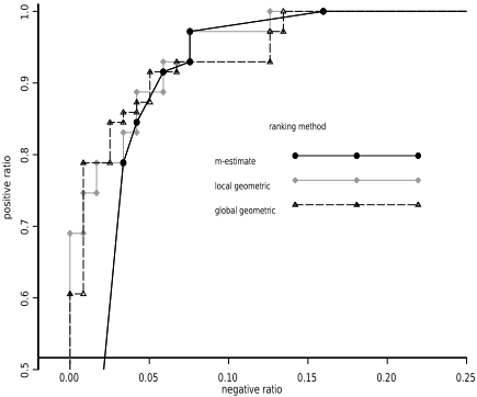
Since DT algorithms are generally designed to maximize accuracy, it is not unreasonable to hypothesize that errors lie near the decision boundary. In a very ideal case, it is even possible to demonstrate that this hypothesis is true.
A DT builds a partition in the input space. In a two class problem, it is possible to associate to a DT a unique function g : E ↦→ {0, 1} such that g(x) is the predicted class of x. (But several decision trees are associated to the same function). We consider an ideal case of statistical decision, where the joint distribution P of observations would be uniform on the graph of the indicator function f of a set S in E = [0, 1]n . We also suppose that the size of all the maximal hypercubes in S and E\S has a lower bound ν > 0 (to prevent pathological situation for S and its boundary). In this case, decision trees built on samples drawn from P can approach f as closely as wanted if the size of the sample can grow indefinitely. For this particular case of function f, errors are located near the decision boundary.
Theorem 3 Proximity of errors. For a DT which associated function g is close enough to f, errors are near the decision boundary ∂g of g.
If we note A the area where f - g ̸= 0 (set of errors), ˙A the interior of A, and if we consider ǫ small enough so that ǫ < ν n , we have:
2
Even if real conditions are very far from this ideal case (in first place, generally f doesn't exist), we can test if the hypothesis of proximity of errors is generally verified. Table 2 shows the mean of the difference of the mean distance of correctly classified cases (hits) and errors from the decision boundary. We also computed for each sample λ, the inverse of the coefficient of variation for the difference of the means defined by (6), where dh and σh are the mean and the standard deviation of the distance of correctly classified examples from the decision boundary, and de and σe the same magnitude for error examples.
Proof. Let x be in ˙A, we consider B(x, d2 ) the maximal hypercube centered at x in its connected component. The volume of B is included into ∫E |f - g|, so we have: dn < ǫ < ν n . So the size of B is smaller than ν and d < n√ǫ. The boundary of B, ∂B, encounters the decision boundary of f - g on at least two meeting points of two different hyperplanes, since B is maximal. If f is not constant on B, then both ∂f and ∂g cross B, and so necessarily d(x, ∂g) < d2 √n. If f is constant on B, since the size of B is smaller than ν, at least one of the meeting point lies on ∂g (otherwise the size of B would be smaller than the lower bound of the maximal balls). So once again d(x, ∂g) ≤ d2 √n < √n n√ǫ. ·
Table 2 shows the percentage of the samples for which λ ≥ 2, which is the 97.5% confidence coefficient under the normal assumption (the test is unilateral). We can see that errors are closer from the decision boundary for a majority of databases. Datasets for which this property is not verified have generally a low mean accuracy (62% for bupa and 69% for sonar). If we consider only the samples for which the accuracy is better than 70%, the proportion shifts to 29% and 50% respectively.
| Database | ∆ of the means | λ | % of samples with λ ≥ 2 |
|---|---|---|---|
| bupa glass iris pima sat | 0.009±0.002 | 0.86±0.12 | 17 |
| 0.038±0.011 | 2.28±0.34 | 51 | |
| ionosphere | 0.037±0.006 | 1.36±0.19 | 35 |
| 0.092±0.003 | 5.34±0.28 | 95 | |
| newThyroid | 0.059±0.002 | 3.46±0.14 | 91 |
| optdigits | 0.542±0.008 | 24.87±1.45 | 100 |
| pendigits | 0.339±0.005 | 24.6±1.24 | 100 |
| 0.036±0.001 | 4.15±0.15 | 94 | |
| 0.135±0.005 | 12.59±0.56 | 100 | |
| segment. | 0.181±0.005 | 7.28±0.2 | 98 |
| sonar | 0.027±0.003 | 1.44±0.14 | 34 |
| vehicle | 0.026±0.004 | 4.75±0.49 | 55 |
| vowel | 0.215±0.003 | 16.88±0.74 | 100 |
| wdbc | 0.113±0.002 | 10.24±0.29 | 100 |
| wine | 0.152±0.004 | 6.73±0.39 | 97.7 |
A corollary of theorem 3 is that if a tree is not accurate, errors may lie everywhere, not only near the decision boundary.
In this case the geometric score cannot be good. So we expect the geometric score to be better with more accurate trees.
4 Experimental Results
4.1 Experimental Design
We have studied the geometric ranking on the database of the UCI repository [Blake and Merz, 1998] that have numerical attributes only and no missing values. We are not directly concerned in this study with the problem of the prevalence of the positive class, since our method doesn't build the decision tree: it applies on the grown tree. So we didn't pay any particular attention to the relative frequency of the classes in the datasets. We chose as positive class either the class with the lowest frequency in the database, either a class which grouped together several classes when it was more logical. When the classes were equiprobable and with no particular meaning we chose it randomly. Although there is a lot of work on the analysis of multi-class problem, for simplicity we have treated multi-class problem as a two class problem (class of the examples were modified before growing the trees).
For each database, we divided 100 bootstrap samples into separate training and test sets in the proportion 2/3 1/3, respecting the prior of the classes (estimated by their frequency in the total database). Even if it is not the best way to build accurate trees for unbalanced dataset or different error costs, here we are not interested in building the most accurate or efficient tree, we just want to study the effect of geometric ranking on pruned trees. For the same reason we grow trees with the default options of j48 (Weka's [Witten and Frank, 2000] implementation of C4.5) although in many cases different options would build better trees. For unpruned trees we disabled the collapsing function.
We used Laplace correction and m-estimate smoothing methods to correct the raw probability estimate at the leaf for reduced-error pruned tree and normal pruned tree. The value of m was chosen such that m × p(c) = 10 where p(c) is the prior probability of the class of interest (as suggested in [Zadrozny and Elkan, 2001]).
We used two different metrics in order to compute the distance from the decision boundary, the Min-Max (MM) metric and the standard (s) metric. Both metrics are defined with the basic information available on the data: An estimate of the range of each attribute i or an estimate of its mean Ei and of its standard deviation si. The new coordinate system is defined by (7).
The parameters of the metric are estimated on each sample. The choice of the metric has a very limited effect on the geometric score; If we measure the difference between the Area Under the ROC curve (AUC) , for each database, it is always less than 2 10-3 ± 9 10-4 , except for the thyroid and vehicle databases (less than 410-3 ) and the glass database (9.510-3 ).
4.2 Comparison between distance-based ranking and smoothing methods
The geometric score is only used to rank the examples without changing the tree structure. It is not used to estimate the posterior probability of an example, so the appropriate measure of performance in that case is the AUC. Table 3 shows the difference between global geometric ranking and Laplace or m-estimate correction at leaf.
| Dataset | Red.-Error pruning | Normal pruning | No pruning | NBTree |
|---|---|---|---|---|
| bupa glass iono. iris letter thyroid optdig. pendig. pima sat segment. sonar vehicle vowel wdbc wine | 0.46±0.48 1.78±0.72 -1.11±0.4 4.69±0.40 0.18±0.09 4.48±0.43 0.53±0.08 0.46±0.04 1.34±0.43 1.01±0.09 8.16±0.75 2.55±0.47 0.35±0.16 4.18±0.34 3.75±0.24 5.35±0.45 | -0.14±0.47 -0.39±0.75 -2.30±0.4 3.85±0.35 0.37±0.07 3.08±0.38 0.34±0.06 0.40±0.03 -0.98±0.25 0.89±0.07 5.27±0.63 1.99±0.51 0.64±0.14 3.09±0.29 2.24±0.18 3.32±0.30 | -0.82±0.50 -1.87±0.73 -2.85±0.42 3.67±0.37 -0.26±0.05 2.54±0.38 0.07±0.06 0.28±0.03 -1.07±0.30 0.46±0.05 5.31±0.64 1.80±0.49 -0.12±0.16 2.83±0.26 2.15±0.18 2.91±0.30 | 0.08 ±0.79 -2.01±0.83 -5.14± 0.72 1.56±0.43 0.40±0.12 -2.13±0.62 -0.12±0.06 0.58±0.05 2.25±0.55 0.97±0.09 3.25±0.61 -5.01±1.03 0.78±0.30 0.78±0.44 2.09±0.22 -0.06±0.25 |
Apart from a few cases, global geometric ranking gives better values than either Laplace or m-estimate correction (with a 95% confidence coefficent). The differences are relatively small (from 0.004 to 0.08), but since they are absolute values the improvement can be important. We have also shown the difference of the AUC between global geometric ranking on reduced-error pruned tree and NBTree.
Table 4 shows the difference between local geometric ranking and smoothing correction at leaf. Local geometric ranking is always better (with a 95% confidence coefficent) than smoothing method alone, except in one case which is not significant. But like for global ranking, the improvement can vary a lot (absolute value from 0.002 to 0.078).
As we said in the theoretical viewpoint section, we expect geometric ranking to outperform smoothing method at the beginning of the ROC curve. To measure the relative behavior of ROC curves for increasing value of the negative ratio, we have computed AUC(x), 0 ≤ x ≤ 0.5, the integral function of the ROC curve, with a 0.001 step value, for the global geometric score (g) and the smoothing correction (s). Table 5 shows for normal pruned trees theshows the maximum absisse value x such that AUCg(y) ≥ AUCs(y) with a confidence coefficient of 0.95 (under the normal assumption) for every y ≤ x. For all smaller values of the negative ratio, the global geometric ranking outperforms the other method (in term of AUC).
We can see in Table 5 that for most bases, the global geometric ranking methods is rather efficient at the beginning of the ROC curve, even when on the total range it performs badly (like for the Pima database, see Table 3). The experiment partially confirms the theoretical viewpoint concerning the fact that geometric score gives interesting results when misclassified examples are near the decision boundary. This is particularly true for the bupa (liver-disorder) and ionosphere databases. Table 2 shows that these datasets doesn't verify the hypothesis of proximity of errors on a majority of samples, and actually the global geometric score give bad results for these datasets.
| Dataset | Reduced-error pruning | Normal pruning | Unpruned |
|---|---|---|---|
| bupa glass iono iris letter thyroid optd. pend. pima sat segment. sonar vehicle vowel wdbc wine | 1.75±0.23 4.21±0.44 0.04±0.29 3.71±0.25 0.19±0.09 3.62±0.39 0.67±0.06 0.34±0.03 2.59±0.26 1.09±0.08 7.78±0.72 3.02±0.29 0.53±0.09 3.83±0.3 3.75±0.22 5.11±0.4 | 0.88±0.09 3.39±0.34 0.51±0.17 3.31±0.26 0.36±0.07 2.70±0.29 0.43±0.04 0.28±0.02 0.87±0.07 0.89±0.06 4.83±0.54 2.81±0.21 0.60±0.07 2.85±0.26 2.14±0.14 3.14±0.26 | 0.69±0.09 2.61±0.31 0.49±0.18 2.92±0.25 0.13±0.02 2.33±0.27 0.27±0.03 0.20±0.02 0.55±0.05 0.45±0.04 4.34±0.49 2.70±0.2 0.49±0.05 2.56±0.23 2.04±0.14 2.80±0.24 |
Concerning the improvement of the geometric ranking when the accuracy of the tree is better, the experiment is not conclusive. If we compute Table 3 and Table 4 for a subset of the samples, the best quartile for tree accuracy, the global geometric ranking is not improved (results are not significant). But local geometric ranking gives always better results than on the total sample, except on the glass and ionosphere database (for which the hypothesis of proximity of errors is not much improved on the subset of the samples).
5 Conclusion
We have presented in this article a geometric method to rank cases that are classified by a decision tree. It applies to every axis-parallel tree that classifies examples with numerical attributes. We were not concerned here with the problem of growing the tree (problem with unbalanced datasets or different misclassification costs which lead to pre-processing of the data or new pruning methods). The geometric method doesn't depend on the type of splitting or pruning criteria that is used to build the tree. It only depends on the shape of decision boundary induced by the tree. It consists in ranking the case according to their distance to the decision boundary, taking into account the class of interest and the class that is predicted by the decision tree. Theoretical arguments suggest that this method is interesting when the misclassified examples lie near the decision boundary, and this was partially confirmed by the experimentation. The combination of geometric ranking and smoothing methods almost always improve the global ranking (measured with the AUC). Different kind of experiment should be performed in order to compare geometric ranling (and particularly local geometric ranking) to NBTree or other algorithm: since the structure of the trees are different, the choice of pruning method can be important.
| MM metric | Standard metric | |||
|---|---|---|---|---|
| Dataset | m-estimate | Laplace | m-estimate | Laplace |
| bupa | 0.001 | 0.001 | 0.001 | 0.001 |
| glass | 0.1 | 0.1 | 0.05 | 0.05 |
| iono | 0.02 | 0.02 | 0.02 | 0.02 |
| iris | ≥ 0.5 | ≥ 0.5 | ≥ 0.5 | ≥ 0.5 |
| thyroid | ≥ 0.5 | ≥ 0.5 | ≥ 0.5 | ≥ 0.5 |
| optdigits | 0.01 | 0.01 | 0.01 | 0.01 |
| pendigits | ≥ 0.5 | ≥ 0.5 | ≥ 0.5 | ≥ 0.5 |
| pima | 0.02 | 0.35 | 0.03 | 0.37 |
| sat | ≥ 0.5 | ≥ 0.5 | ≥ 0.5 | ≥ 0.5 |
| segment. | ≥ 0.5 | ≥ 0.5 | ≥ 0.5 | ≥ 0.5 |
| sonar | ≥ 0.5 | ≥ 0.5 | ≥ 0.5 | ≥ 0.5 |
| vehicle | ≥ 0.5 | ≥ 0.5 | ≥ 0.5 | ≥ 0.5 |
| vowel | ≥ 0.5 | ≥ 0.5 | ≥ 0.5 | ≥ 0.5 |
| wdbc | ≥ 0.5 | ≥ 0.5 | ≥ 0.5 | ≥ 0.5 |
| wine | ≥ 0.5 | ≥ 0.5 | ≥ 0.5 | ≥ 0.5 |
The main limit of the method is that it is limited to numerical attributes. It could be extended to ordered attributes, but without the definition of a utility function it cannot be used with attributes that have unordered modalities.
Further work is in progress in order to understand more precisely when the geometric ranking should perform well. Following the idea from [Smyth et al., 1995], we think that density estimator could be used on the distance itself rather than on the attribute of the cases, in order to deal with 1dimension estimator (which are very efficient). Another interesting point is the definition of a geometric score for real multi-class problem (with no particular class of interest). Actually the algorithm that computes the distance to the decision boundary computes already the distance of an example to the different classes, so these distances could be used for that purpose.
@inproceedings{ijcai2005p195,
  title     = {Ranking Cases with Decision Trees: a Geometric Method that Preserves Intelligibility},
  author    = {Alvarez, Isabelle and Bernard, Stephan},
  booktitle = {Proceedings of the Nineteenth International Joint Conference on
               Artificial Intelligence, {IJCAI-05}},
  publisher = {International Joint Conferences on Artificial Intelligence},
  pages     = {635--639},
  year      = {2005},
  url       = {https://ijcai.org/proceedings/2005/195},
}
TY - CPAPER TI - Ranking Cases with Decision Trees: a Geometric Method that Preserves Intelligibility AU - Alvarez, Isabelle AU - Bernard, Stephan T2 - Proceedings of the Nineteenth International Joint Conference on Artificial Intelligence, IJCAI-05 PB - International Joint Conferences on Artificial Intelligence PY - 2005 SP - 635 EP - 639 UR - https://ijcai.org/proceedings/2005/195 ER -Copied
Machine-readable versions of this paper, for tools and AI agents:





