Dynamic Control Of Plans With Temporal Uncertainty

1 Introduction

Simple Temporal Networks [Dechter et al., 1991] have proved useful in planning and scheduling applications that involve quantitative time constraints (e.g. [Laborie and Ghallab, 1995; Muscettola et al., 1998b]) because they allow fast checking of temporal consistency. However this formalism does not adequately address an important aspect of real execution domains: the time of occurrence of some events may not be under the complete control of the execution agent. For example, when a spacecraft commands an instrument or interrogates a sensor, a varying amount of time may intervene before the operation is completed. In cases like this, the execution agent does not have freedom to select the precise time delay between events in accord with the timing of previously executed events. Instead, the value is selected by Nature independently of the agent's choices. This can lead to constraint violations during execution even if the Simple Temporal Network appeared consistent at plan generation time.

The problem of constraint satisfaction for temporal networks with uncertainty was first addressed formally in [Vidal and Ghallab, 1996; Vidal and Fargier, 1999]. In this setting, the question of temporal feasibility goes beyond mere consistency to encompass issues of "controllability." Essentially, a network is controllable if there is a strategy for executing

Thierry Vidal

LGP/ENIT

47, av d'Azereix - BP 1629 F-65016 Tarbes cedex - FRANCE

thierry@enit.fr

the timepoints under the agent's control that satisfies all requirements, in all situations involving the uncontrolled timepoints. The previous work has identified three primary levels of controllability. In Strong Controllability, there is a static control strategy that is guaranteed to work in all cases. In Weak Controllability, for all situations there is a "clairvoyant" strategy that works if all uncertain durations are known when the network is executed. The most interesting controllability property from a practical point of view is Dynamic Controllability, where it is assumed that each uncertain duration becomes known (is observed) after it has finished, and the property requires a successful strategy that depends only on the past outcomes.

In previous work, algorithms have been presented for checking Strong and Weak Controllability, and Strong Controllability has been shown to be tractable, while Weak Controllability is co-NP-complete [Vidal and Fargier, 1999; Morris and Muscettola, 1999]. However, Dynamic Controllability has proved difficult to analyze, primarily because of a time asymmetry where a control decision may depend on the past but not on the future. In this paper we present efficient constraint propagation methods for checking Dynamic Controllability. These explicitly add constraints that are implicit in the Dynamic Controllability property. With these additional constraints, Dynamic Controllability checking reduces to a form of consistency checking that turns out to be polynomial. The derived constraints are also used to guide an effective execution strategy.

2 Background

We review the definitions of Simple Temporal Network [Dechter et al., 1991], and Simple Temporal Network with Uncertainty [Vidal and Fargier, 1999].

A Simple Temporal Network (STN) is a graph in which the edges are labelled with upper and lower numerical bounds. The nodes in the graph represent temporal events or timepoints, while the edges correspond to constraints on the durations between the events. Formally, an STN may be described as a 4-tuple < N,E, l, u > where N is a set of nodes, E is a set of edges, and l : E → IR ∪ {-∞} and u : E → IR ∪ {+∞} are functions mapping the edges into extended Real Numbers, that are the lower and upper bounds of the interval of possible durations. Each STN is associated with a distance graph [Dechter et al., 1991] derived from the upper and lower bound constraints. An STN is consistent if and only if the distance graph does not contain a negative cycle, and this can be determined by a single-source shortest path propagation such as in the Bellman-Ford algorithm [Cormen et al., 1990]. To avoid confusion with edges in the distance graph, we will refer to edges in the STN as links.

A Simple Temporal Network With Uncertainty (STNU) is similar to an STN except the links are divided into two classes, contingent links and requirement links. Contingent links may be thought of as representing causal processes of uncertain duration; their finish timepoints, called contingent timepoints, are controlled by Nature, subject to the limits imposed by the bounds on the contingent links. All other timepoints, called executable timepoints, are controlled by the agent, whose goal is to satisfy the bounds on the requirement links. We assume the durations of contingent links vary independently, so a control procedure must consider every combination of such durations.

Thus, an STNU is a 5-tuple < N,E, l, u,C >, where N,E, l, u are as in a STN, and C is a subset of the edges: the contingent links, the others being requirement links. We assume 0 < l(e) < u(e) < ∞ for each contingent link e. 1

An STNU may be regarded as an STN by ignoring the distinction between contingent links and requirement links. This allows us to apply STN terminology and concepts, such as AllPairs shortest-path calculations, to STNUs.

In addition, choosing one of the allowed durations for each contingent link may be thought of as reducing the STNU to an ordinary STN. Thus, an STNU determines a family of STNs, as in the following definition.

Suppose Γ = < N, E, l, u, C > is an STNU. A projection [Vidal and Ghallab, 1996] of Γ is a Simple Temporal Network derived from Γ where each requirement link is replaced by an identical STN link, and each contingent link e is replaced by an STN link with equal upper and lower bounds [b, b] for some b such that l(e) ≤ b ≤ u(e).

Given a fixed STNU < N, E, l, u, C >, a schedule T is a mapping

where T(x), written Tx here, is called the time of time-point x. A schedule is consistent if it satisfies all the link constraints. From a schedule, we can determine the durations of all contingent links that finish prior to a timepoint x. (This may be viewed as a partial mapping from C to IR.) We call this the prehistory of x with respect to T , denoted by T≺x.

Then an execution strategy S is a mapping

where P is the set of projections and T is the set of schedules. An execution strategy S is viable if S(p) is consistent (w.r.t. p) for each projection p.

We are now ready to define the various types of controllability, essentially following [Vidal, 2000].

An STNU is Weakly Controllable if there is a viable execution strategy. This is equivalent to saying that every projection is consistent.

1 If l(e) = u(e), there is no uncertainty and we may as well replace e by a requirement link.

An STNU is Strongly Controllable if there is a viable execution strategy S such that

for each executable timepoint x and projections p1 and p2. Thus, a Strong execution strategy assigns a fixed time to each executable timepoint irrespective of the outcomes of the contingent links.

An STNU is Dynamically Controllable if there is a viable execution strategy S such that

for each executable timepoint x and projections p1 and p2. Thus, a Dynamic execution strategy assigns a time to each executable timepoint that may depend on the outcomes of contingent links in the past, but not on those in the future (or present). This corresponds to requiring that only information available from observation may be used in determining the schedule. We will use dynamic strategy in the following for a (viable) Dynamic execution strategy.

Networks where two contingent links have the same finishing point are clearly not Dynamically Controllable. Because of this, and for certain technical reasons (following [Morris and Muscettola, 2000]), we will exclude such networks in the remainder of this paper.

It is easy to see from the definitions that Strong Controllability implies Dynamic Controllability, which in turn implies Weak Controllability. Strong Controllability is known to be tractable and Weak Controllability is known to be co-NPcomplete. In this paper, we investigate the status of Dynamic Controllability. Note that a na¨ıve algorithm for checking this property is hyperexponential since it requires searching for an execution strategy that is both dynamic and viable, while a method described in [Vidal, 2000] requires worst case exponential space.

The following terminology will be useful in the subsequent discussion. A contingent link is squeezed if the other constraints (including the other contingent links) imply a strictly tighter lower bound or upper bound for the link. An STNU is pseudo-controllable if it is consistent and none of the contingent links are squeezed.

If a network is pseudo-controllable then all the edges arising from contingent links are shortest paths. Thus, the contingent links survive unchanged in the AllPairs shortest-path graph (abbreviated as the AllPairs graph). Note that pseudocontrollability can be determined in polynomial time by computing the AllPairs graph.

It is easy to see that every Weakly Controllable network is pseudo-controllable since a squeezed contingent link would imply a projection that is not consistent. However, the converse is not true in general.

Even for a STNU that was originally pseudo-controllable, it is possible for a contingent link to be squeezed during execution (which may be viewed as augmenting the network with additional constraints). In this paper, we will make use of results from [Morris and Muscettola, 2000]. These guarantee that a contingent link cannot be squeezed during execution under certain circumstances. Essentially, upper bounds can only be squeezed by propagations through links with non-negative upper bounds, and lower bounds can only be squeezed by propagations through links with positive lower bounds. Even in these cases, squeezing cannot occur if the relevant bound is dominated by that of the contingent link, which essentially means the bound at issue is redundant. If the dominance relations are such that no contingent link can be squeezed, then the network is safe. A safe network can be executed like an ordinary STN, and thus is Dynamically Controllable.

3 Triangular Reductions

A starting point for resolving the issue of Dynamic Controllability is to consider triangular STNU networks, i.e., networks involving three timepoints and including a contingent link, as shown in figure 1. Here AC is a contingent link with bounds [x, y], while AB and BC are requirement links with bounds [p, q] and [u, v] respectively. This notation for contingent and requirement links will be used in subsequent diagrams. The contingent link AC is called the focus of the triangle. We will also assume that the triangular networks we consider are pseudo-controllable and have been placed in AllPairs form, so every edge is a shortest path. It follows that [u, v] ⊆ [x - q, y - p], which implies [p, q] ⊇ [y - v, x - u].

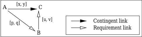
We will derive a number of results concerning additional tightenings or reductions of the bounds that must be obeyed by any schedule resulting from a dynamic strategy (i.e., any S(p) for any projection p, in the notation of the previous section). These will vary according to cases involving the signs of the [u, v] bounds.

1. First suppose that v < 0. We call this the Follow case, since the lower bound of CB (i.e., BC reversed) is -v and hence B follows C. Then the network is Dynamically Controllable since C has already been observed at the time B is executed. In fact, it may be executed like an ordinary STN since any propagation will go from C to B and not vice versa. Thus, the network is safe and no tightening is needed.
2. Next consider the case where u ≥ 0. We call this the Precede case, since B occurs before or simultaneously with C. Then no information about C is available to B. In this case, we claim that AB can be tightened to [y - v, x - u]. Suppose there is a projection p that a dynamic strategy maps to a schedule T with TB - TA < y - v. Since C is not in T≺B or T≺A, TB and TA cannot depend on AC. Therefore TA and TB are unchanged if the projection is mutated to a projection p′ where AC equals y. But then we have BC = TC -TB = (TC -TA)-(TB-TA) > y-(y-v) = v, so the BC constraint will be violated. Thus, TB-TA ≥ y-v. A similar argument shows TB - TA ≤ x - u. After the

tightening of AB to [y - v, x - u] (or equivalently BA to [u - x, v - y]), the BC bounds are dominated (redundant) since [u - x, v - y] + [x, y] = [u, v]. Thus, the network is safe provided it is still pseudo-controllable.

1. The most interesting case occurs when u < 0 and v ≥ 0, which we call the Unordered case, since B may or may not follow C. However, suppose B does not follow C and TB -TA < y-v. As in the previous case, there is then a projection where the BC constraint is violated. We conclude that, for a dynamic strategy, B cannot be executed at any time before y - v after A if C has not already occurred. This is a conditional constraint on AB, depending on the time of occurrence of C. It may also be viewed as a ternary constraint on A,B, and C, which we call a wait since B must wait until either C occurs or the wait expires at y - v after A.

First, there is one subcase for which the conditional constraint turns out to be unconditional, which is when y-v ≤ x. Then C cannot occur before the wait expires, so we can simply raise the lower bound of AB to y - v. We will call this the unconditional Unordered reduction.

In the truly conditional subcase where x < y - v, an obvious idea is to branch on the conditional and consider separately two possibilities. First if it turns out that AC < y - v (in which case C occurs first and B follows), the network is safe if pseudo-controllable as in the Follow case. Otherwise if AC ≥ y - v then AB ≥ y - v also, which gives BA an upper bound of v - y. Thus, the BC upper bound of v is dominated (redundant). Since the lower bound u is negative, the network is safe if pseudo-controllable [Morris and Muscettola, 2000]. Observe that in either case B occurs later than x after A, so without branching we can raise the lower bound of AB to x. We will call this the general Unordered reduction.

We see above that assuming a dynamic strategy may lead to a tightening of the constraint bounds. If the tightening produces a violation of pseudo-controllability, then the original network was not Dynamically Controllable. On the other hand, if the network remains pseudo-controllable after the tightening (in the general Unordered case we must verify this for both possibilities), then the triangular network is safe and thus Dynamically Controllable [Morris and Muscettola, 2000]. Thus, the tightenings give a procedure for determining Dynamic Controllability of triangular networks.

4 Local vs Global Dynamic Controllability

To test a general STNU network for Dynamic Controllability, we can construct the AllPairs graph, which may be regarded as a combination of triangular subnetworks. Triangles that involve a contingent link may be viewed as instances of figure 1. If a triangle contains two contingent links, 2 then we consider it twice, with each contingent link in turn playing the role of focus, and the other being treated as a requirement link. Any tightening propagates to neighbour triangles until quiescence of the network is reached. The only problem arises with Unordered cases: if we branch on the conditionals as discussed in the previous section, we end up with a combinatorial search, which we prefer to avoid. Instead we use only the two non-branching Unordered reductions discussed earlier, so the resulting iterative algorithm is deterministic and polynomial. (But the network is then not necessarily safe.)

2 Triangles with three contingent links cannot occur, since we have excluded coincident finishing points.

This propagation algorithm with no search may be viewed as a local Dynamic Controllability checking procedure. Since it applies to triangles, this is similar to a path-consistency algorithm in a classical constraint network such as a STN. Hence, we call this local property 3-Dynamic Controllability and call the resulting algorithm 3DC. As with any local filtering algorithm, the process is sound: if it fails, then at least one triangle is not Dynamically Controllable and therefore the whole network is not.

However, it is incomplete as shown by the example in figure 2. We invite the reader to verify that the triangles are all quiescent under the deterministic reductions considered above; therefore the network is stable under 3DC.

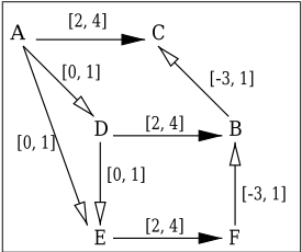
Now consider the subnetwork ACDB. It is not difficult to see that a dynamic strategy requires AD = 1. Similarly, DE must be 1. But that causes a violation of the AE link. Hence the network is not Dynamically Controllable. 3 This example also shows that 3DC does not compute the minimal network, i.e., the network in which values not belonging to any dynamic strategy have been removed (for instance here AD would be tightened to [1,1]). A checking algorithm should ideally produce this minimality property, which is desirable for execution purposes. Nevertheless, 3DC is an efficient technique to rule out a wide variety of networks.

5 Regression of Waits

The incompleteness of 3DC might suggest we should reconsider a combinatorial search. However, we have not exhausted the possibilities of obtaining deterministic reductions from the Unordered cases. If the ternary constraint corresponding to the Unordered wait is used directly, then no branching is necessary. Moreover, this ternary constraint can be treated somewhat like a binary constraint. Suppose we have a wait condition that requires B to wait for C until time t after A. We will indicate that by placing a <C, t> annotation on the AB link. Note that if it is impossible for C to occur before t (for example if the lower bound of AC is greater than t), then the <C, t> wait becomes a true lower bound of t on AB. This corresponds to the unconditional Unordered reduction discussed earlier.

3 Note that this example is Weakly Controllable, as can be seen by considering the worst case projection for each cycle.

Now consider figure 2 again. The triangle ABC is an Unordered case, so AB receives a <C, 3> wait. This is not unconditional since the lower bound of AC is 2. Now consider triangle ADB with this new label on AB. Suppose C has not occurred yet and D is executed before 1 time unit after A. In the projection where DB equals 2, B will then occur before 3 time units after A. If C still has not occurred by then, the wait on AB will be violated. In other words, the wait on AB can be regressed through DB to obtain a derived wait on AD, still relative to C: <C, 1> . This, happily, is an unconditional wait since C cannot occur before time 2, which produces a lower bound of 1 on AD and leads to a resolution of the example. One can notice as well that we achieve the hoped-for minimal network. That leads us to the following result.

Lemma 1 (Regression) Suppose a link AB has a wait <C, t> , where t is less than or equal to the upper bound of AC. Then (in a schedule resulting from a dynamic strategy):

• (i) If there is any link DB (including AB itself) with upper bound w, then we can deduce a wait <C, t - w> on AD.

(ii) If t ≥ 0 and if there is a contingent link DB with lower bound z, where B ̸= C, then we can deduce a wait <C, t - z> on AD.

Proof: Consider (i) first. Suppose D occurs before t - w after A and C has not occurred yet. From the upper bound w on DB, it follows that B must occur before w+t-w = t. But this violates the wait on AB in the projection where C occurs at its upper bound (which is ≥ t). We conclude that D cannot occur before t - w after A unless C has already occurred.

Now consider (ii). If t ≥ 0, then B must be later than A. Suppose D occurs before t-z after A and C has not occurred yet. Then neither A nor D can depend on the outcomes of AC or DB. Thus, we can consider a mutated projection where DB finishes at z and AC finishes at its upper bound. This leads to a violation of the AB wait. ✷

Note that (i) and (ii) are both applicable to contingent links but (ii) gives a more restrictive (longer) wait.

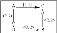
Iterated regression amounts to a new type of propagation, where waits are spread to other links. The propagated waits can be examined for any unordered reductions, which place additional ordinary constraints throughout the network. For example, consider figure 3. Intuitively, we can see this is not Dynamically Controllable because the waits in the worst case will cause an incursion on the AC lower bound (assuming the upper bounds of the AP,DQ,BR contingent links are all at least 2). First we can regress the <R, 2> wait through procedure DynamicallyControllable? (network W)

1. Compute the All-Pairs graph for W.
2. If W is not pseudo-controllable then return false.
3. Select any triangle such that v is non-negative. Introduce any tightenings required by the Precede case and any waits required by the Unordered case.
4. Do all possible regressions of waits, while converting unconditional waits to lower bounds. Also introduce lower bounds as provided by the general reduction.
5. If steps 2 and 3 do not produce any new (or tighter) constraints, then return true, otherwise go to 1.

Figure 4: DC Checking Algorithm

AC, which gives a wait of <R, -3> on BA. This gives rise to (unconditional case) a lower bound of -3 on BA, which is equivalent to an upper bound of +3 on AB. Now we can regress the <Q, 2> wait on DB through AB, which gives a <Q,-1> on DA, giving rise to a +1 upper bound on AD. Finally, we regress the <P, 2> wait on AD through AD itself, which gives a <P, 1> wait on AA. Now the general reduction ensures a positive lower bound on AA, which is a direct inconsistency. Thus, we have reduced the lack of Dynamic Controllability to a violation of consistency.

6 Dynamic Checking and Execution

We are now ready to introduce the algorithm for determining Dynamic Controllability, summarized in figure 4. It is just an enhancement of 3DC with wait regressions and hence is still a local algorithm, but now we can show it is complete.

We prove completeness by presenting a dynamic execution algorithm and showing that it is viable if the DC checking algorithm reports success. For simplicity, we will assume the execution takes place in the AllPairs graph of the tightened network, although performance could be improved by transforming it to a minimum dispatchable graph as in [Muscettola et al., 1998a]. The execution is essentially the same as for an ordinary STN except for adding a requirement to respect the waits. For this purpose, we only consider waits <C, t> where t satisfies l(C) < t ≤ u(C). Note that waits with t ≤ l(C) are converted to lower bounds, while waits with t > u(C) are equivalent to those with t = u(C). (Since l(C) > 0 by definition, the waits enforced by the algorithm are all positive.)

The execution algorithm is shown in figure 5. We assume there is some start timepoint that is constrained to be before every other timepoint. (If necessary, one can be added.) In step 2, a timepoint is live if the current time is within the timepoint's bounds. It is enabled if all timepoints required to be executed before it (by links with positive lower bounds) have already been executed [Muscettola et al., 1998a].

It is clear that this algorithm provides a strategy where the decisions depend only on the past. The issue is whether any constraints are violated. Properties of STNs guarantee that they can be executed incrementally [Muscettola et al., 1998a]. Therefore, only the special features introduced for STNUs need be considered. The following are the possible ways in which the execution might fail.

• A deadlock might occur where a wait lasts forever.
• A wait might be forcibly aborted.

procedure Execute (network W)

1. Perform initial propagation from the start timepoint.
2. Immediately execute any executable timepoints that have reached their upper bounds.
3. Arbitrarily pick an executable timepoint TP that is live and enabled and not yet executed, and whose waits, if any, have all been satisfied.
4. Execute TP. Halt if network execution is complete. Otherwise, propagate the effect of the execution.
5. Advance current time, propagating the effect of any contingent timepoints that occur, until an executable timepoint becomes eligible for execution under 1 or 2.
6. Go to 1.

Figure 5: DC Network Execution

• A propagation might squeeze a contingent link.

An example of a potential deadlock is when AC and DB are contingent links with a <C, t1> wait on AD and a <B, t2> wait on DA. More generally, a deadlock requires a cycle of links, each of which is labelled with a wait or a positive lower bound. However, the waits <C, t> enforced by the execution algorithm satisfy l(C) < t ≤ u(C) (see above). These imply a positive lower bound of l(C) by the general reduction. Thus, we would have a cycle where each link has a positive lower bound. This corresponds to an inconsistency in the network that would be detected by step 1 of the DC checking algorithm. The other possibilities are considered in the following lemmas.

Lemma 2 Suppose a network has successfully passed the DC checking algorithm. Then the first failure that occurs during the DC execution cannot be an aborted wait.

Proof: Suppose the first failure is an aborted wait, and the earliest time this occurs involves a wait <C, t> on a link AB. As pointed out above, this wait must be positive, so the link AB will have a positive lower bound. First we note that B obviously cannot be the start timepoint.

There are now two cases to consider. In the first case, the wait is aborted because step 1 required an immediate execution of B. Consider the timepoint D (possibly the start) whose execution initiated the propagation that produced the upper bound of B. Note the regression of <C, t> through DB produces a wait of <C, t - u(DB)> on AD. If t - u(DB) ≤ l(AC), the checking algorithm places it as an unconditional lower bound on AD. Otherwise, <C, t -u(DB)> is an earlier wait that is enforced by the execution algorithm. In either case, D does not occur until t-u(DB) after A. Suppose b and d are the upper bounds of B and D, respectively, and a is the time of execution of A. Then (d - a) ≥ (t - u(DB)). Since b = d + u(DB), it follows that (b - a) ≥ t. This contradicts the assumption that the wait was terminated.

The second case involves the possibility that B is a contingent timepoint. (Thus, the execution is not controlled by the agent). Suppose EB is a contingent link with bounds [x, y]. Again we can regress the wait through EB getting <C, t-x> on AE. Since E is earlier than B, the latter wait must be satisfied. Thus, the duration of AE is greater than t - x. Since x is the minimum duration of EB, it follows that AB is greater than t -x+x = t, i.e., the wait is satisfied after all. ✷

Lemma 3 Suppose a network has successfully passed the DC checking algorithm. Then the first failure that occurs during DC execution cannot be a squeezing of a contingent link.

Proof: Suppose the earliest failure is the squeezing of a contingent link AC that has bounds [x, y]. This must occur during a propagation that either raises the lower bound of AC or lowers the upper bound. However, the triangular reductions ensure that AC dominates adjacent links with finishing point C, except for the case of links BC with negative lower bound u and non-negative upper-bound v such that y -v > x (the conditional Unordered case). This means the only possibility for a squeezing is an upper-bound propagation along some such BC. However, the existence of such a BC would cause the checking algorithm to place a <C, y -v> wait on AB. If C occurs before B then there is no propagation from B to C. Otherwise, the enforcement of the wait by the execution algorithm ensures that B is not executed before y - v after A. Thus, the upper bound propagated along BC will be TB+v ≥ (TA+y-v)+v = TA+y, so AC is not squeezed. ✷

Theorem 1 Dynamic Controllability can be determined in deterministic polynomial time.

Proof: Lemmas 2 and 3 demonstrate that the execution algorithm successfully executes networks that are verified by the checking algorithm. Thus, the Dynamic Controllability checking algorithm is complete. As noted earlier, the algorithm is also sound since the added constraints were derived from the assumption of Dynamic Controllability.

The individual tightenings are clearly polynomial, and convergence is assured because the domains of the constraints are strictly reduced by the tightenings. The only issue is how long the convergence takes. A crude upper bound can be obtained by assuming a fixed level of precision δ and finite bounds (say between ±β) on all links. If there are η links, then after at most 2ηβ/δ reductions, some domain would become empty. This bound grows polynomially with the size of the problem. ✷

It is worth pointing out that the execution algorithm presented here preserves maximum flexibility, since the additional tightenings and waits were all required by Dynamic Controllability. (In contrast to the approach, for example, of adding waypoints [Morris and Muscettola, 1999], which surrenders some flexibility.) Another interesting point is that the execution algorithm allows the selection of any execution time within prescribed limits, without impairing the success of the dynamic strategy. Therefore the incremental application of the DC propagation ensures that the values remaining in the domains are consistent with the dynamic strategy. In other words, the DC checking algorithm produces the minimal network in the sense described earlier.

7 Conclusions

Dynamic Controllability is polynomial! That is certainly the main contribution of this paper, since this property, needed in many real-world applications such as planning and scheduling, was expected to be much harder.

Moreover, the proposed method is directly applicable to the STNU (as opposed to a previous technique that needed a translation into a finite-state automaton model [Vidal, 2000]), and is inspired by classical constraint satisfaction techniques. We have presented a local Dynamic Controllability algorithm based on triangle reductions, and have shown that non-binary constraints that were inherent in the problem give rise to binary constraints through a regression process. We have also proven this local controllability algorithm is complete with respect to Dynamic Controllability of the global network.

We believe our contribution will be valuable in the design of new constraint programming packages that handle temporal uncertainty and will help pave the way to effective realtime execution systems that incorporate such uncertainties.