Managing Temporal Uncertainty Through Waypoint Controllability

1 Introduction

Simple Temporal Networks [Dechter et al., 1991] have proved useful in Planning and Scheduling applications that involve metric time (e.g. [Bienkowski and Hoe bel, 1998; Muscettola et al., 1998a]). However this formal­ ism does not adequately address an important aspect of real execution domains: the occurrence time of some events may not be under the complete control of the execution agent. For example, when a spacecraft com­ mands an instrument or interrogates a sensor, a vary­ ing amount of time may intervene before the operation is completed. In cases like this, the execution agent cannot select the precise time delay between events in accord with the timing of previously executed events. Instead, the value is selected by Nature independently of the agent's choices. This can cause inconsistencies at execution time even if the Simple Temporal Network appeared consistent at plan generation time. The prob­ lem of control of temporal networks with uncertainty was first addressed formally in [Vidal and Ghallab, 1996] and [Vidal and Fargier, 1997].

Nicola Muscettola Recom Technologies Mail Stop 269-2 NASA Ames Research Center Moffett Field, CA 94035 mus@ptolemy. arc.nasa.gov

In practice, temporal uncertainty is usually eliminated by padding each uncertain interval with a flexible wait period. For example, a task duration may be modeled as the upper bound of the task's possible executions. In this case, the event at the end of a task does not repre­ sent the time at which the task actually ends. Instead, it constitutes a waypoint, i.e., a time by which we can guar­ antee that the task has ended. Synchronization with re­ spect to waypoints can now proceed without uncertainty and Simple Temporal Networks are completely adequate. Although this use of waypoints provides a workable so­ lution to the problem of execution uncontrollability, its indiscriminate application may not be desirable or pos­ sible. For example, it may obstruct tight synchroniza­ tion with respect to follow-on requirements. Moreover, it may not be possible to add a wait period after each un­ certain delay if several uncontrollable delays are causally connected.

In this paper we introduce Waypoint Controllability, a general framework for a formal analysis of when net­ works that incorporate uncontrollable delays can be suc­ cessfully executed. Waypoint controllability generalizes the concepts of Strong and Weak Controllability [Vidal and Ghallab, 1996; Vidal and Fargier, 1997]. Roughly speaking, Strong Controllability supplies a guarantee of a fixed execution that works irrespective of the outcomes of the uncontrollable delays, while the absence of Weak Controllability means that there are some outcomes for which no execution will work. Subject to restrictions on the type of network, an algorithm is presented in [Vi­ dal and Ghallab, 1996] that determines Strong Control­ lability in deterministic polynomial time. It is shown in [Vidal and Fargier, 1997] that the negation of Weak Controllability is in NP and it is conjectured that the problem is NP-Complete.

We prove here that the negation of Weak Controlla­ bility is indeed NP-Complete. This complexity result applies also to Waypoint Controllability, of which Weak Controllability is a special case. Sufficient conditions are presented for the tractability of Waypoint Controllabil­ ity. From these, we are able to derive the tractability of Strong Controllability while relaxing the restrictions in [Vidal and Ghallab, 1996] . We also provide a prop­ agation algorithm for determining Waypoint Controllability. Finally we discuss the relationship between Way­ point Controllability and Dynamic Controllability, where knowledge of uncontrollable delays is updated during ex­ ecution.

2 Preliminaries

We assume the reader is broadly familiar with Simple Temporal Networks [Dechter et al., 1991]. The definition is briefly reviewed here to set the stage for subsequent developments.

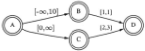
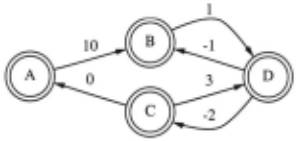
A Simple Temporal Network (STN) is a graph in which the edges are labelled with upper and lower numerical bounds. The nodes in the graph represent temporal events or timepoints, while the edges correspond to con­ straints on the durations between the events. Formally, an STN may be described as a 4-tuple < N, E, l, u > where N is a set of nodes, E is a set of edges, and l : E -+ lll U { -oo} and u : E -+ lll U { +oo} are func­ tions mapping the edges into extended Real Numbers. Figure 1 shows an example of an STN. Figure 2 shows the corresponding distance graph [Dechter et al., 1991], which is an alternate representation useful for mathe­ matical analysis. Note that lower bounds are negated to give the lengths of the reverse edges. Edges of infinite length are omitted. (Given a distance graph, one can also find a corresponding STN, so the representations are interchangeable.) An STN is consistent if and only if the distance graph does not contain a negative cycle.

Controllability problems [Vidal and Ghallab, 1996; Vidal and Fargier, 1997] arise in STNs where the edges, which we will call links, are divided into two classes, causal links and requirement links. The causal links are regarded as representing intervals whose duration is con­ trolled by Nature, subject to the limits imposed by the upper and lower bounds. The timepoints are regarded as variables. The goal is that they should have values that satisfy all the requirement links as well as whatever values are chosen by Nature for the causal links.

Definition 1 A Simple Temporal Network with Uncer­ tainty (Vidal and Fargier, 1997} (STNU) is a 5-tuple < N,E,l,u,C >,where N,E,l,u are as in a STN, and C is a subset of the edges. The edges in C are called the causal links, and the other edges are the requirement links. We require 0 < l(e) < u(e) for each causal link e.

The requirement that the lower bounds of causal links be positive corresponds to the assumption that causal influences propagate only forward in time. (Only theo­ rem 5 actually makes use of this.) Also notice that if a link e is rigid (i.e., l(e) = u(e)), then there is little point in making e a causal link, since there is no uncertainty in the outcome.

Each set of choices made by Nature for the causal links may be thought of as reducing the STNU to an ordinary STN. Thus, an STNU determines a family of STNs, as in the following definition.

Definition 2 Suppose r = < N, E, l, u, C > is an STNU. A projection (Vidal and Ghallab, 1996} of r is a Simple Temporal Network derived from r where each requirement link is replaced by an identical STN link, and each causal link e is replaced by an STN link with equal upper and lower bounds [b, b] for some b such that l(e) ~ b ~ u(e).

A boundary projection (Vidal and Fargier, 1 997} is one where, for each causal link e, the above b is chosen so that b = l(e) orb= u(e).

The simplest type of controllability property is con­ cerned with whether some outcomes of the causal choices render it impossible to satisfy the requirements.

Definition 3 An STNU is Weakly Controllable (Vidal and Ghallab, 1 996} if every one of its projections is a consistent STN. If an STNU is not Weakly Controllable, we will say it is Weakly Uncontrollable.

It is shown in [Vidal and Fargier, 1997] that Weak Un­ controllability can be determined in non-deterministic polynomial time, and that in fact the checking may be limited to the boundary projections. (Recall that consis­ tency of a distance graph may be checked in polynomial time by the Bellman-Ford-Moore algorithm [Cormen et al., 1990].)

Theorem 1 (Vidal and Fargier, 1997) If any pro­ jection is inconsistent, then a boundary projection is in­ consistent.

3 Weak Uncontrollability NP-Completeness

We now address the issue of showing Weak Uncontrol­ lability is NP-Complete. Since it is known from [Vidal and Fargier, 1997] that the problem is inNP, it remains to show it is NP-Hard.

Theorem 2 Weak Uncontrollability is NP-Hard.

Proof: We show this by reduction of the 3-Coloring Problem, which is known to be NP-Complete [Cormen et al., 1990].

Our goal will be to construct a mapping from coloring problems to STNU distance graphs such that a solution to the coloring problem maps to a negative cycle in some projection of the STNU, and vice versa. For expository purposes, we adopt the widget approach of [Cormen et al., 1990].

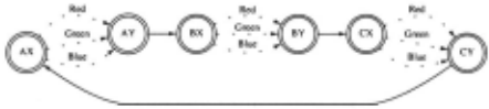
The first widget describes how nodes and colors from the coloring problem are represented in the STNU dis­ tance graph. This is illustrated in figure 3 for a coloring problem with 3 nodes {A, B, C}. The node A from the coloring problem maps to a pair of nodes AX and AY. The three possible colors of A correspond to three con­ current paths from AX to AY as shown. (The labels Red, Green, and Blue do not actually appear in the temporal network; they are merely shown for the convenience of the reader.) A similar mapping is shown for nodes B and C.

Suppose the coloring problem has n nodes {A1 , .. . , An} (listed in some arbitrary order). We link all the node widgets to form a cycle by adding temporal edges AiY -t Ai+lX for 1 :S i < n and AnY -t A1X. This is also illustrated in figure 3. Note that each complete set of color choices determines a cycle in the network. Conversely, each cycle selects a single color for each node.

So far, we have not assigned lengths to the distance graph edges. The final edge in the STNU distance graph (e.g., CY -t AX in figure 3) is given a length of -1. Apart from the mutex widgets (discussed below), all the other edges have zero length. Notice that, so far , all combinations of color choices give rise to slightly negative (value -1) cycles in the distance graph.

Our next task is to represent in the temporal net­ work the mutual exclusion constraints determined by the edges of the coloring problem. (Nodes connected by an edge must have different colors.) We will do this by set­ ting up "mutex" widgets between color paths that cor­ respond to conflicting color choices. Figure 4 shows how to make two color paths mutually exclusive from nega­ tive cycles. Here L is a positive number large enough so that if a path through the widget has length L or greater, then it cannot possibly be on a negative cycle. (Setting L = +2 suffices here.) Notice the edges P -t Q and Q -t Pare each shown with two values for the edge length; these correspond to a causal link from P to Q with bounds [2L, 4L], and the different lengths are for the different boundary projections.

There are four paths through the mutual exclusion widget that may potentially lie on negative cycles: the two color paths A1 -t P -t Q -t A2 and B1 -t Q -t P -t B2; and the two short paths A1 -t P -t B2 and B1 -t Q -t A2. Notice that both of the short paths pick up a value of L, so they are definitely not on nega­ tive cycles. The two color paths may or may not be on negative cycles.

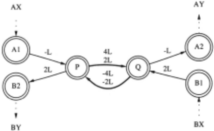
Recall that to check for Weak Uncontrollability, we need only consider boundary projections, where the P -t Q causal link has a rigid length of either 2L or 4L. In the distance graph, this corresponds to values of either +2L and -2L, respectively, or +4L and -4L, respectively, for the forward (from P to Q) and backward (from Q to P) edges. In the first case, the color path from A1 to A2 has distance 0, while that from B1 to B2 is 2L. In the second case, the path from B1 to B2 has distance 0 while that from A1 to A2 has distance 2L, i.e., the values are reversed. Notice that in either case, at most one of the two color paths can be on a negative cycle, i.e., they mutually exclude each other from such cycles.

The same node in the color graph may participate in several color constraints. In the temporal network, we represent these by mutual exclusion widgets connected in series, as illustrated in figure 5, where each "mutex" box indicates a mutual exclusion widget between the AX -t AY color path and some other color path (not shown) .

This completes the construction. Now suppose the coloring problem has a solution. We can use the color choices to determine a cyclic path in the distance graph that passes through each mutual exclusion widget at most once, and then traverses the -1 edge. Since there is a projection that sets the chosen passages through the mutual exclusion widgets to zero distance, the cycle will have a total length of -1. Thus, the constructed STNU is not Weakly Controllable. Conversely, suppose there is a negative cycle in some projection. This cannot include any of the short paths, since if it did, the cycle would be non-negative. Consequently, the cycle includes only color paths, as illustrated in figure 3. Thus, it selects a single color for each color node. If two of the selections were in conflict, then the cycle would pass through some mutex widget twice, which contradicts the assumption that the cycle is negative. Thus, the color selection pro­ vides a solution to the coloring problem.

This reduction of the 3-Coloring Problem shows Weak Uncontrollability is NP-Complete. 0

4 Waypoint Controllability

Now we consider a form of controllability in which we distinguish a subset of events, called waypoints, whose timing is set independently of the causal outcomes.

Definition 4 Let r = < N, E, l, u, C > be an STNU. Suppose W is a non-empty subset of N. We say f is Waypoint Controllable with respect to W if there is a fixed assignment of time values to the nodes in W that can be extended to a solution in every projection of r. The nodes in W are called waypoints.

In [Vidal and Ghallab, 1996], the property of Strong Controllability is defined similarly, except a specific set of waypoints is used. Their definition corresponds to a waypoint set C8 U (N \ Ce), where Cs and Ce are the sets of start and end points, respectively, of the causal links. However, Strong Controllability lacks flexibility. For ex­ ample, if two causal links are chained (the end of one is the start of the other), Strong Controllability requires that both the start and end of the earlier causal link be waypoints. However, a fixed assignment to those points cannot be consistent with varying durations of a flexible causal link. Thus, the network is not Strongly Control­ lable. This limits the usefulness of Strong Controllability in many networks; in the example above, some other set of waypoints, for instance N \ Ce, may be more realistic.

Note that Weak Controllability is a special case of Waypoint Controllability where the waypoint set is a sin­ gleton, since it is always possible to select a single node and give it a fixed value that is extendible to a solution in every consistent projection.

We will shortly prove a useful characterization of Way­ point Controllability. However, some additional defini­ tions are needed. Given an STNU r and a set of way­ points W, we can define a Simple Temporal Network S(f, W) as follows. The set of nodes of S(f, W) is W. Between every pair of nodes x and y in W, we place a distance graph edge e whose length is given by

where Pis the set of projections of r and ov(x, y) is the shortest-path distance from x toy in the distance graph of projection p. This leads to the following result, which may be regarded as a generalization of the result in [Vi­ dal and Ghallab, 1996] concerning Strong Controllability in a restricted network.

Theorem 3 r is W aypoint Controllable with respect to W if and only if it is Weakly Controllable and S(f, W) is a consistent STN.

Proof: Suppose r is Waypoint Controllable with re­ spect to W. Then there is a fixed assignment s : W -+ lR that can be extended to a solution in every projec­ tion of r. It follows that every projection has a so­ lution, i.e., r is Weakly Controllable. It also follows that s(y)- s(x) :::::; Ov(x, y) for every projection p, where Op gives the shortest-path distances as before. Hence, s(y)- s(x) :::::; min{ov(x, y) I p E P}. Thus, s gives a solution to S(f, W).

Conversely, assuming s is a solution to S(f, W), the argument can be reversed to deduce that s(y)- s(x) :::::; op(x, y) for every projection p, and every x andy in W. By Weak Controllability, every projection is consistent, so by Decomposability [Dechter et al., 1991], s can be extended to a solution for every projection. 0

It can be shown that in the min{ Op(x, y) I p E P} minimizations, the set P may be restricted to boundary projections without affecting the minimum value. Nev­ ertheless, the cardinality of P is generally exponential in the size of the problem. Indeed, the proof of Theorem 2 can be adapted to show that the minimization problem is NP-hard. However, theorem 3 leads to a propaga­ tion algorithm for computing Waypoint Controllability, and there are important special cases where it runs in polynomial time.

5 Propagation Algorithm

The propagation algorithm is an elaboration of the ap­ proach used for checking STN consistency [Dechter et al., 1991; Cormen et al., 1990], and requires that every node be reachable from the initial node, which must be selected to be a waypoint. The basic idea is that we can perform a separate propagation for each projection until we reach a waypoint. At the waypoint, the propa­ gated values for the different projections can be merged, and only the minimum value carried forward. The pro­ cess continues with new independent propagations to the next waypoint, and so on. Notice that the updates at the waypoints simulate an ordinary STN propagation in S(f, W). Both STN inconsistency and Weak Uncontrol­ lability imply a negative cycle, so propagation to qui­ escence is a reliable indicator of controllability by theo­ rem 3.

Actually, we can do even better if we observe that large segments of the propagation are.the same for projections that are closely related. This suggests sharing the work of propagation between the projections. We do this by associating a tag with each propagated value. The tag carries a description of which causal links have been tra­ versed so far, and which of the boundary values were used in the traversals. We say one tagged value subsumes another if its tag is as general (i.e., its causal choices are a subset of the other) and its value is as good (less than or equal to the other). Subsumed tagged values are sub­ ject to deletion. Otherwise, the tagged propagations do

procedure Propagate-Controllability begin end Queue <- {}; Propagate-Value (0, {}, Initial-Node, Queue); while Queue is Non-Empty do begin end <X,V,T> <-Pop (Queue); if Bellman-Ford bound is exceeded then report Uncontrollability and halt; for each causal edge E:X->Y from X do begin end if E/2 does not occur in T then Propagate-Value (V+lengthl(E), T U {E/1}, Y, Queue); if E/1 does not occur in T then Propagate-Value (V+length2(E), T U {E/2}, Y, Queue); for each non-causal edge E:X->Y from X do Propagate-Value (V+length(E), T, Y, Queue); procedure Propagate-Value (Val, Tag, X, Queue) begin end TV <- (if X is Waypoint then <Val,{}> else <Val,Tag>; if TV is not subsumed by an existing tagged value of X then begin Delete tagged values of X subsumed by TV; Add TV to tagged values of X; Add <X,val(TV),tag(TV)> to Queue; end

not interact until they reach a waypoint, where the tags are reset to empty. The usual Bellman-Ford cutoff termi­ nates the propagation in cases where the network is not controllable. Figure 6 shows a pseudo-code description of the algorithm. Note that length! (E) and length2 (E) are the lengths of E corresponding to the two boundary values, and the choice descriptors E/1 and E/2 indicate which of those was used in the propagation.

Similarly to the ordinary STN case, the propagation algorithm can be modified to propagate upper and lower time bounds. Thus, it potentially provides not just a single solution for the waypoints, but a flexible set of acceptable time assignments with the same decompos­ ability property as for an ordinary STN. An execution algorithm can make use of this flexibility [Tsamardinos et al., 1998] to help manage contingencies that are unantic­ ipated, in addition to the formally represented uncertain durations considered here.

Note that in general the number of possible tags grows exponentially with the number of causal links. Thus, in the worst case, the time and space complexities are exponential. Fortunately, the waypoints can serve to limit the complexity, as seen in the following result.

Theorem 4 Suppose M is the maximum number of causal links that can occur in a path with no interior waypoints. Then the complexity of the Waypoint Con­ trollability propagation algorithm is O(M 2 2 2 MINIIEI).

Proof: Since the tags get reset at waypoints, the size of tags is limited to the number of causal links encountered between waypoints. Under the condition of the theorem, at most 2M different tagged values can reside at any node. The update across an edge then requires at most

0(2 2 M) subsumption tests, where each test can be done in O(M 2 ) time. The Bellman-Ford bound restricts the number of edge updates to INI·IEI [Cormen et al., 1990]. Thus, the total complexity is O(M 2 2 2 MINIIEI). D

Corollary 4.1 The algorithm can determine Strong Controllability in polynomial time.

Proof: The waypoint set used in Strong Controllability has a waypoint at the start of each causal link. Thus, at most two causal links can occur in a path between waypoints, so M is bounded for this class of problems. D

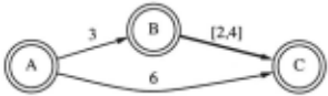
We remark that a "no U-turn" restriction [Muscettola et al., 1998b] is insufficient to avoid interference between projections in computing minimum distance. For exam­ ple, in figure 7, where B -+ C is a causal link, the prop­ agation A -+ B -+ C would produce a value of 5 at C, which blocks the propagation A -+ C -+ B that would provide a shorter distance of 2 from A to B. This kind of interference is avoided by the tag mechanism used here.

6 Dynamic Controllability

Note that Waypoint Controllability requires the setting of times for non-waypoint events to depend on the causal outcomes. However, this is only feasible in practice if in­ formation about the causal outcomes is available in time. One scenario is where precise information about causal outcomes is obtained by observation when they occur. This corresponds to a property called Dynamic Control­ lability defined in [Vidal and Fargier, 1997]. Informally, an STNU is Dynamically Controllable if there is a map­ ping from projections to solutions such that the partial solution up to any time depends only on the durations of the causal outcomes that have completed by that time. We are interested in conditions under which Waypoint Controllability implies Dynamic Controllability.

The following conditions will be relevant. Consider the distance graph of a Waypoint Controllable network. We say a node x is insulated from another node y if every path from y to x passes through a waypoint. (Note that a waypoint is therefore insulated from every node.) A node x is downstream from a node y if, in every projection, there is a path of negative length from x to y. (We will also say y is upstream of x in this case.) Note that if x is downstream from y, then x must occur later than y in any solution of any projection. Finally, a node x is protected from y if x is either downstream from y or is insulated from y. This leads to the following result.

Theorem 5 Let r be an STNU that is Waypoint Con­ trollable with respect to some set of waypoints. Suppose every node x is either itself a causal link endpoint, or is protected from every causal link endpoint. Then r is Dynamically Controllable.

Proof: From the definition of Waypoint Controllabil­ ity, there is a fixed assignment of times to the waypoints that is consistent with every projection. Consider any projection p. We can obtain a solution of p by propa­ gating from the fixed times of the waypoints, and then choosing the latest possible time for each node [Dechter et al., 1991]. (Ensured to be finite by adding a source vertex as in [Cormen et al., 1990, page 541].) This de­ fines a mapping Ill from projections to solutions.

Let x be any node. Suppose p1 and p2 are two projec­ tions that agree on causal outcomes that are completed no later than x. Then they must agree on outcomes of causal links whose endpoint is upstream from x. We wish to show that ll!(p1) and ll!(p2) must agree on the timing of x. We prove this by induction on the partial ordering imposed by the downstream relation, which allows us to suppose by induction that ll!(p1) and ll!(p2) agree on the timing of all nodes upstream of x.

First consider the case where x is the endpoint of a causal link e. Let x' be the startpoint of e. By the definition of STNU, l(e) > 0. Thus, x' is upstream of x. It follows that ll!(p1) and ll!(p2) agree on the timing of x'. Also p1 and p2 agree on the outcome of e,_ since it is completed no later than x. Thus, ll!(p1) and ll!(p2) agree on the timing of x.

Otherwise, x is not the endpoint. of a causal link. Let e be any causal link, and suppose its endpoint is y . By the condition of the theorem, x is either downstream of y or is insulated from y. In the former case, y is upstream of x, so by the inductive hypothesis ll!(p1) and ll!(p2) agree on y. Thus, any value propagated from y to x will be the same for p1 and p2. If on the other hand x is insulated from y, then any propagation from y to x is blocked by the fixed assignments given the waypoints. Thus, x will have the same propagated window for both p1 and p2, and so Ill will assign x the same time value in both cases.

It follows that the value of x depends only on causal outcomes that are completed no later than x. Thus, r is Dynamically Controllable. 0

Corollary 5.1 (Vidal and Fargier, 1997) Strong Controllability implies Dynamic Controllability.

Proof: Strong Controllability corresponds to a set of waypoints such that every node is either a causal link endpoint or a waypoint. In the latter case it is automat­ ically insulated from every node. 0

7 Closing Remarks

Waypoint Controllability provides a useful analysis tool that can be used by a planner to decide whether grant­ ing the executive access to uncertain events compromises controllability of a flexible plan. We have shown that the cost of controllability analysis can be affordable, pro­ vided that the planner judiciously manages the place­ ment of uncontrollable links in the plan topology.

One important consequence of Waypoint Controllabil­ ity is the possibility of devising more general and princi­ pled guidelines on the introduction of wait periods in a plan. The end time point of a suitable wait link can be made a waypoint. Therefore, appropriately located wait periods can partition a plan into compartments that are insulated from each other as far as the effects of uncer­ tain events are concerned.

Previous work on Strong Controllability restricted the plan topologies for which controllability is guaranteed, and severely limited the extent to which an executive can react to uncertain events. For example, Strong Con­ trollability does not allow an executive to have access to an event linking two uncontrollable tasks. Waypoint Controllability shows that such limitations can be lifted provided that small subnetworks of uncontrollable links (with arbitrary topology) are insulated from the rest of the plan through the appropriate use of wait periods.

Acknowledgments

We thank Ari Jonsson and Pandu Nayak for suggestions to improve the presentation.