
Search on High Degree Graphs
Proceedings of the Seventeenth International Joint Conference on Artificial Intelligence. Pages 266-273.
© 2001 International Joint Conferences on Artificial Intelligence
Abstract
We show that nodes of high degree tend to occur infrequently in random graphs but frequently in a wide variety of graphs associated with real world search problems. We then study some alternative models for randomly generating graphs which have been proposed to give more realistic topologies. For example, we show that Watts and Strogatz’s small world model has a narrow distribution of node degree. On the other hand, Barab ́asi and Albert’s power law model, gives graphs with both nodes of high degree and a small world topology. These graphs may therefore be useful for benchmarking. We then measure the impact of nodes of high degree and a small world topology on the cost of coloring graphs. The long tail in search costs observed with small world graphs disappears when these graphs are also constructed to contain nodes of high degree. We conjecture that this is a result of the small size of their “backbone”, pairs of edges that are frozen to be the same color.
- [Achlioptas et al., 2000] D. Achlioptas, C. Gomes, H. Kautz, and B. Selman. Generating satisfiable problem instances. In Proc. of 17th Nat. Conf. on AI. 2000.
- [Barabási and Albert, 1999] A-L. Barabási and R. Albert. Emergence of scaling in random networks. Science, 286:509-512, 1999.
- [Barabási et al., 1999] A-L. Barabási, R. Albert, and H. Jeong. Mean-field theory for scale-free random networks. Physica A, 272:173-187, 1999.
- [Brelaz, 1979] D. Brelaz. New methods to color the vertices of a graph. Communications of ACM, 22:251-256, 1979.
- [Culberson and Gent, 2000] J. Culberson and I.P. Gent. Frozen development in graph coloring. Theoretical Com- puter Science, 2001. To appear.
- [Fujita et al., 1993] Masayuki Fujita, John Slaney, and Frank Bennett. Automatic generation of some results in finite algebra. In Proc. of the 13th IJCAI, pages 52-57. 1993. IJCAI
- [Gent et al., 1999] I.P. Gent, H. Hoos, P. Prosser, and T. Walsh. Morphing: Combining structure and random- ness. In Proc. of the 16th Nat. Conf. on AI. 1999.
- [Gomes et al., 1997] C. Gomes, B. Selman, and N. Crato. Heavy-tailed distributions in combinatorial search. In G. Smolka, editor, Proc. of 3rd Int. Conf. on Principles and Practice of Constraint Programming (CP97), pages 121-135. Springer, 1997.
- [Gomes et al., 1998] C. Gomes, B. Selman, K. McAloon, and C. Tretkoff. Randomization in backtrack search: Ex- ploiting heavy-tailed profiles for solving hard scheduling problems. In The 4th International Conference on Artifi- cial Intelligence Planning Systems (AIPS'98), 1998.
- [Hogg, 1996] T. Hogg. Refining the phase transition in com- binatorial search. Artificial Intelligence, 81(1-2):127-154, 1996.
- [Monasson et al., 1998] R. Monasson, R. Zecchina, S. Kirk- patrick, B. Selman, and L. Troyansky. Determining computational complexity for characteristic 'phase transi- tions'. Nature, 400:133-137, 1998.
- [Parkes, 1997] A. Parkes. Clustering at the phase transition. In Proc. of the 14th Nat. Conf. on AI, pages 340-345. 1997.
- [Render, 1998] S. Render. How popular is your paper? An empirical study of the citation distribution. European Physical Journal B, 4:131-134, 1998.
- [Walsh, 1999] T. Walsh. Search in a small world. In Pro- ceedings of 16th IJCAI. Artificial Intelligence, 1999.
- [Watts and Strogatz, 1998] D.J. Watts and S.H. Strogatz. Collective dynamics of 'small-world' networks. Nature, 393:440-442, 1998.
References were extracted automatically from the PDF and may contain errors.
Full text extracted automatically from the PDF; figures, tables and equations may differ. The PDF is the version of record.
1 Introduction
How does the topology of graphs met in practice differ from uniform random graphs? This is an important question since common topological structures may have a large impact on problem hardness and may be exploitable. Barab´asi and Albert have shown that graphs derived from areas as diverse as the World Wide Web, and electricity distribution contain more nodes of high degree than are likely in random graphs of the same size and edge density [Barab´asi and Albert, 1999]. As a second example, Redner has shown that the citation graph of papers in the ISI catalog contains a few nodes of very high degree [Render, 1998]. Whilst 633,391 out of the 783,339 papers receive less than 10 citations, 64 are cited more than 1000 times, and one received 8907 citations. The presence of nodes with high degree may have a significant impact on search problems. For instance, if the constraint graph of a scheduling problem has several nodes with high degree, then it may be difficult to solve as some resources are scarce. As a second example, if the adjacency graph in a Hamiltonian circuit problem has many nodes of high degree, then the problem may be easy since there are many paths into and out of these nodes, and it is hard to get stuck at a "dead-end" node. Search heuristics like Brelaz's graph coloring heuristic [Brelaz, 1979] are designed to exploit such variation in node degree.
This paper is structured as follows. We first show that nodes of high degree tend to occur infrequently in random graphs but frequently in a wide variety of real world search problems. As test cases, we use exactly the same problems studied in [Walsh, 1999]. We then study some alternative models for randomly generating graphs which give more nonuniform graphs (specifically Barab´asi and Albert's power law model, Watts and Strogatz's small world model, and Hogg's ultrametric model). Finally, we explore the impact of nodes of high degree on search and in particular, on graph coloring algorithms.
2 Random graphs
Two types of random graphs are commonly used, the a0 ✁ ✄ ✆ and the a0 ✁ ✄ ✝ models. In the a0 ✁ ✄ ✆ model, graphs with ✞ nodes and ✟ edges are generated by sampling uniformly from the ✞ ✠ ✞ ☞ ✍ ✏ ✒ ✔ possible edges. In the a0 ✁ ✄ ✝ model, graphs with ✞ nodes and an expected number of ✖ ✞ ✠ ✞ ☞ ✍ ✏ ✒ ✔ edges are generated by including each of the ✞ ✠ ✞ ☞ ✍ ✏ ✒ ✔ possible edges with fixed probability ✖ . The two models have very similar properties, including similar distributions in the degree of nodes. In a random a0 ✁ ✄ ✝ graph, the probability that a node is directly connected to exactly ✤ others, ✖ ✠ ✤ ✏ follows a Poisson distribution. More precisely,
where ✞ is the number of nodes, ✖ is the probability that any pair of nodes are connected, and ✱ is ✠ ✞ ☞ ✍ ✏ ✖ , the expected node degree. As the Poisson distribution decays exponentially, nodes of high degree are unlikely.
In this paper, we focus on the cumulative probability, ✸ ✠ ✤ ✏ which is the probability of a node being directly connected to ✤ or less nodes:
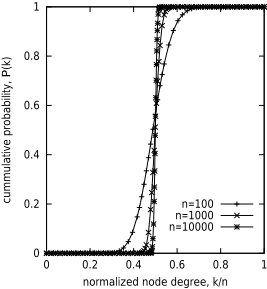
Whilst ✖ ✠ ✤ ✏ is smoothly varying for randomgraphs, it can behave more erratically on real world graphs. The cumulative probability, which is by definition monotonically increasing, tends to give a clearer picture. Figure 1 shows that the cumulative probability against the normalized degree for random graphs rapidly approaches a step function as ✞ increases. The degree of nodes therefore becomes tightly clustered around the average degree.
3 Real world graphs
We next studied the distribution in the degree of nodes found in the real world graphs studied in [Walsh, 1999].
3.1 Graph coloring
We looked at some real world graph coloring problems from the DIMACS benchmark library. We focused on the register allocation problems as these are based on real program code. Figure 2 demonstrates that these problems have a very
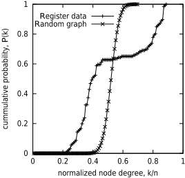
skewed distribution in the degree of their nodes. Other problems from the DIMACS benchmark library gave very similar cumulative probability distributions for the degree of their nodes. Compared to random graphs of the same size and edge density, these register allocation problems have a number of nodes that are of much higher and lower degree than the average. For example, the node of maximum degree in Figure 2 is directly connected to 89% of the nodes in the graph. This is more than twice the average degree, and there is less than a 1 in 4 million chance that a node in a random graph of the same size and edge density has degree as large as this. On the other hand, the node of least degree has less than half the average degree, and there is less than a 1 in 7 million chance that a node in a random graph of the same size and edge density has degree as small as this. The plateau region in the middle of the graph indicates that there are very few nodes with the average degree. Most nodes have either higher or lower degrees. By comparison, the degrees of nodes in a random graph are tightly clustered around the average. A similar plateau region around the average degree is seen in most of the register allocation problems in the DIMACS benchmark library.
3.2 Time-tabling
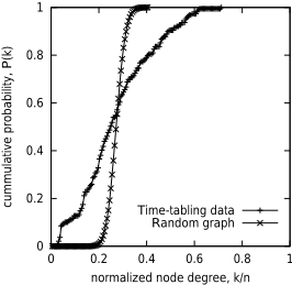
Time-tabling problems can be naturally modelled as graph coloring problems, with classes represented by nodes and time-slots by colors. We therefore tested some real world time-tabling problems from the Industrial Engineering archive at the University of Toronto. Figure 3 demonstrates that problems in this dataset also have a skewed distribution in the degree of their nodes. Other benchmark problems from this library gave very similar curves. Compared to random graphs with the same number of nodes and edges, these timetabling problems have a number of nodes that have much higher and lower degree than the average. For example, the node of maximum degree in Figure 3 is directly connected to 71% of the nodes in the graph. This is nearly three times the average degree, and there is less than a 1 in ✍ ❅ ❇ ❈ chance that a node in a random graph of the same size and edge density has degree as large as this. On the other hand, the node of least degree has approximately one tenth of the average degree, and there is less than a 1 in ✍ ❅ ✾ ❊ chance that a node in a random graph of the same size and edge density has degree as small as this. [Walsh, 1999] suggests that sparse problems in this dataset have more clustering of nodes than the dense problems. However, there was no obvious indication of this in the distribution of node degrees.
3.3 Quasigroups
A quasigroup is a Latin square, a ✟ by ✟ multiplication table in which each entry appears just once in each row or column. Quasigroups can model a variety of practical problems like sports tournament scheduling and the design of factorial experiments. A number of open questions in finite mathematics about the existence (or non-existence) of quasigroups with particular properties have been answered using model finding and constraint satisfaction programs [Fujita et al., 1993]. Recently, a class of quasigroup problems have been proposed as a benchmark for generating hard and satisfiable problem instances for local search methods [Achlioptas et al., 2000].
An order ✟ quasigroup problemcan be represented as a binary constraint satisfaction problem with ✟ ❇ variables, each with a domain of size ✟ . The constraint graph for such a problem consists of ✔ ✟ cliques, one for each row and column, with each clique being of size ✟ . Each node in the constraint graph is connected to ✔ ✠ ✟ ☞ ✍ ✏ other nodes. Hence, ✖ ✠ ✤ ✏ ✪ ✍ if ✤ ✪ ✔ ✠ ✟ ☞ ✍ ✏ and 0 otherwise, and the cumulative probability ✸ ✠ ✤ ✏ is a step function at ✤ ✪ ✔ ✠ ✟ ☞ ✍ ✏ . As all nodes in the constraint graph of a quasigroup have the same degree, quasigroups may suffer from limitations as a benchmark. For example, the Brelaz heuristic [Brelaz, 1979] (which tries to exploit variations in the degree of nodes in the constraint graph) may perform less well on quasigroup problems than on more realistic benchmarks in which there is a variability in the degree of nodes.
4 Non-uniform randommodels
As the a0 ✁ a80 ✆ and a0 ✁ ✄ ✝ models tend to give graphs with a narrow distribution in the degree of nodes, are there any better models for randomly generating graphs? In this section, we look at three different random models, all proposed by their authors to give more realistic graphs.
4.1 Small world model
Watts and Strogatz showed that graphs that occur in many biological, social and man-made systems are often neither completely regular nor completely random, but have instead a "small world" topology in which nodes are highly clustered yet the path length between them is small [Watts and Strogatz, 1998]. Such graphs tend to occur frequently in real world search problems [Walsh, 1999]. To generate graphs with a small world topology, we randomly rewire a regular graph like a ring lattice [Watts and Strogatz, 1998; Gent et al., 1999]. The ring lattice provides nodes that are highly clustering, whilst the random rewiring introduces short cuts which rapidly reduces the average path length. Unfortunately, graphs constructed in this manner tend not to have a wide distribution in the degree of nodes, and in particular are unlikely to contain any nodes of high degree. For small amounts of rewiring, ✖ ✠ ✤ ✏ peaks around the lattice degree, and converges on the Poisson distribution found in random graphs for more extensive rewiring.
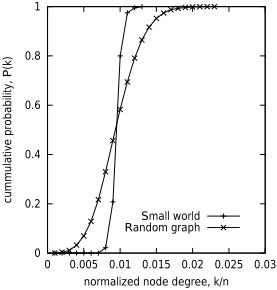
In Figure 4, we plot the cumulative probability for the node degrees of graphs generated to have a small world topology by randomly rewiring a ring lattice. Small world graphs have a distribution of node degrees that is narrower than that for random graphs with the same number of nodes and edges. Due to the lack of variability in the degree of nodes, these small world graphs may have limitations as a model of real world graphs. The absence of nodes of high degree is likely to impact on search performance. For instance, heuristics like Brelaz which try to exploit variations in node degree are likely to find these graphs harder to color than graphs with a wider variability in node degree. Can we find a model with a variability in the node degree that is similar to that seen in the real world graphs studied in the previous section?
4.2 Ultrametric model
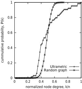
To generate graphs with more realistic structures, Hogg has proposed a model based on grouping the nodes into a tree-like structure [Hogg, 1996]. In this model, an ultrametric distance between the ✞ nodes is defined by grouping them into a binary tree and measuring the distance up this tree to a common ancestor. A pair of nodes at ultrametric distance ❘ is joined by an edge with relative probability ✖ ❙ . If ✖ ✪ ✍ , graphs are purely random. If ✖ ❲ ✍ , graphs have a hierarchical clustering as edges are more likely between nearby nodes. Figure 5 gives the cumulative probability distribution for the node degrees in a graph generated with an ultrametric distance using the model from [Hogg, 1996]. There is a definite broadening of the distribution in node degrees compared to random graphs. Nodes of degree higher and lower than the average occur more frequently in these ultrametric graphs than in random graphs. For example, one node in the ultrametric graph is connected to all the other nodes. This node has more than twice the average degree, and there is less than a 1 in 3 million chance that a node in a random graph of the same size and edge density has degree as large as this. On the other hand, the node of least degree has just over half the average degree, and there is less than a 1 in 500 chance that a node in a random graph of the same size and edge density has degree as small as this. Ultrametric graphs thus provide a better model of the distribution of node degrees. However, they lack a small world topology as nodes are not highly clustered [Walsh, 1999]. Can we find a model which has both a small world topology (which has shown to be common in real world graphs) and a large variability in the node degree (which has also been shown to be common)?
4.3 Power lawmodel
Barab´asi and Albert have shown that real world graphs containing nodes of high degree often follow a power law in which the probability ✖ ✠ ✤ ✏ that a node is connected to ✤ others is proportional to ✤ ✭ ❪ where ❫ is some constant (typically around 3) [Barab´asi and Albert, 1999]. Redner has shown that highly cited papers tend to follow a Zipf power law with exponent approximately -1/2 [Render, 1998]. It follows from this result that the degree of nodes in the citation graph for highly cited papers follows a power law with ✖ ✠ ✤ ✏ proportional to ✤ ✭ ❴ . Such power law decay compares to the exponential decay in ✖ ✠ ✤ ✏ seen in random graphs.
To generate power law graphs, Barab´asi and Albert propose a model in which, starting with a small number of nodes (✞ ❈ ), they repeatedly add newnodes with ✟ (✟ ❵ ✞ ❈ ) edges. These edges are preferentially attached to nodes with high degree. They suggest a linear model in which the probability that an edge is attached to a node ✿ is ✤ ✼ ✒ ❛ ❝ ✤ ❝ where ✤ ❝ is the degree of node ❞ . Using a mean-field theory [Barab´asi et al., 1999], they show that such a graph with ✞ nodes has:
That is, ✖ ✠ ✤ ✏ is proportional to ✤ ✭ ❪ where ❫ ✪ ❢ . Note that ✖ ✠ ✤ ✏ is also proportional to ✟ ❇ , the square of the average degree of the graph. In the limit of large ✞ , ✖ ✠ ✤ ✏ ❤❥ ❇ ✆ ❦ ✲ ♠ . The presence of non-linear terms in the preferential attachment probability will change the nature of this power law scaling and may be a route to power laws in which the scaling exponent is different to 3.
We propose a minor modification to this model to tackle the problem that the average degree ✟ is bounded by the size of the initial graph ✞ ❈ . This will hinder the construction of high density graphs (which were not uncommon in the previous section). We suggest connecting an edge to a node ✿ with probability ♣ a113 a115 ✠ ✍ ✉ ✟ ✤ ✼ ✒ ❛ ✼ ✤ ✼ ✏ . Each new node is then connected to the graph by approximately ✟ edges on average. This modification is similar to moving from the a0 ✁ a80 ✆ to the a0 ✁ a80 ✝ model of random graphs.
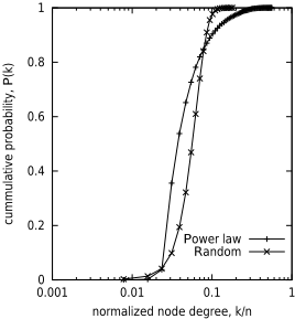
In Figure 6, we plot the cumulative probability for the degree of nodes in graphs generated by this modified model. As with the ultrametric graphs, we observe a definite broadening of the distribution in node degrees compared to random graphs. Nodes of degree higher and lower than the average occur more frequently in these power law graphs than in random graphs. For example, the node of maximum degree is directly connected to 70% of the nodes in the graph. This is more than three times the average degree, and there is less than a 1 in ✍ ❅ ✾ ✈ chance that a node in a random graph of the same size and edge density has degree as large as this. On the other hand, the node of least degree has nearly one fifth of the average degree, and there is less than a 1 in ✍ ❅ ✇ chance that a node in a random graph of the same size and edge density has degree as small as this. Unlike random graphs in which the distrib ① ution sharpens as we increase the size of graphs, we see a similar spread in the distribution of node degrees as these graphs are increased in size.
Ideally, we want like a method for generating graphs that gives graphs with both nodes of high degree and a small world topology. The nodes of high degree generated by the (modified) Barab´asi and Albert model are likely to keep the average path length short. But are the nodes likely to be tightly clustered? Table 1 demonstrates that these graphs tend to have a small world topology as the graph size is increased.
| ✞ | ② | ② ③ ④ ✁ ❙ | ⑥ | ⑥ ③ ④ ✁ ❙ | ⑦ |
|---|---|---|---|---|---|
| 16 | 1.00 | 1.00 | 1.00 | 1.00 | 1.00 |
| 32 | 1.24 | 1.24 | 0.81 | 0.77 | 1.05 |
| 64 | 1.57 | 1.56 | 0.57 | 0.43 | 1.35 |
| 128 | 1.77 | 1.78 | 0.39 | 0.24 | 1.62 |
| 256 | 1.93 | 1.89 | 0.25 | 0.12 | 2.12 |
| 512 | 2.07 | 2.10 | 0.16 | 0.06 | 2.58 |
5 Search
Graphs generated by the modified Barab´asi and Albert model have both a broad distribution in degree of their nodes and a small world topology. These are both features which are common in real world graphs but rare in random graphs. These graphs may therefore be good benchmarks for testing graph coloring algorithms. They may also be useful for benchmarking other search problems involving graphs (e.g. for generating the constraint graph in constraint satisfaction problems, the adjacency graph in Hamiltonian circuit problems, ...)
Unfortunately coloring graphs generated by the (modified) Barab´asi and Albert model is typically easy. Most heuristics based on node degree can quickly (in many cases, immediately) find a ✟ ❸ ✍ -coloring. In addition, a ✟ -clique can be quickly found within the nodes of high degree showing that a ✟ ❸ ✍ -coloring is optimal. A simple fix to this problem is to start with an initial graph which is not a clique. This initial graph could be a ring lattice as in [Watts and Strogatz, 1998; Walsh, 1999], or the inter-linking constraint graph of a quasigroup as in [Gent et al., 1999]. In both cases, we observe similar results. The choice of the initial graph has little effect on the evolution of nodes of high degree. In addition, starting from a ring lattice or the constraint graph of a quasigroup promotes the appearance of a small world topology. As in [Achlioptas et al., 2000; Gent et al., 1999], we generate problems with a mixture of regular structure (from the initial graph) and randomness (from the addition of new nodes).
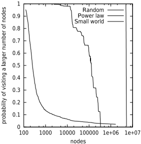
In Figure 7, we plot the distribution in search costs for coloring graphs with either a power law scaling in their node degree, a small world topology or a purely random topology. To find optimal colorings, we use an algorithm due to Mike Trick which is based upon Brelaz's DSATUR algorithm [Brelaz, 1979]. Unlike small world graphs, power law graphs do not display a long tail in the distribution of search costs. Whilst power law graphs are easier to color than random graphs, there is a larger spread in search costs for power law graphs than for random graphs. The absence of a long tail means that there are less benefits with these power law graphs for a randomization and rapid restart strategy [Gomes et al., 1997; 1998] compared to small world graphs [Walsh, 1999].
5.1 Backbones
Recent efforts to understand the hardness of satisfiability problems has focused on "backbone" variables that are frozen to a particular value in all solutions [Monasson et al., 1998]. It has been shown, for example, that hard random 3-SAT problems from the phase transition have a very large backbone [Parkes, 1997]. Backbone variables may lead to thrashing behaviour since search algorithms can branch incorrectly on them. If these branching mistakes occur high in the search tree, they can be very costly to undo. The idea of backbone variable has been generalized to graph coloring [Culberson and Gent, 2000]. Since any permutation of the colors is also a valid coloring, we cannot look at nodes which must take a given color. Instead, we look at nodes that cannot be colored differently. As in [Culberson and Gent, 2000], two nodes are frozen in a ✤ -colorable graph if they have the same color in all valid ✤ -colorings. No edge can occur between two nodes that are frozen. The backbone is simply the set of frozen pairs.
The power law graphs generated by the modified Barab´asi and Albert model in Figure 7 had very small backbones. Indeed, in many cases, there are only one or two pairs of nodes in the backbone. At the start of search, it is therefore hard to color incorrectly any of the nodes in one of these power law graphs. This helps explain the lack of a long tail in the distribution of search costs. By comparison, the small world graphs had backbones with between fifty and one hundred pairs of nodes in them. At the start of search, it is therefore easy to color incorrectly one of nodes. This gives rise to a long tail in the distribution of search costs for backtracking algorithms like Brelaz's DSATUR algorithm.
6 Conclusions
We have shown that nodes of high degree tend to occur infrequently in random graphs but frequently in a wide variety of real world search problems. As test cases, we used exactly the problem studied in [Walsh, 1999]. We then studied some alternative models for randomly generating nonuniform graphs. Watts and Strogatz's small world model gives graphs with a very narrow distribution in node degree, whilst Hogg's ultrametric model gives graphs containing nodes of high degree but lacks a small world topology. Barab´asi and Albert's power law model combines the best of both models, giving graphs with nodes of high degree and with a small world topology. Such graphs may be useful for benchmarking graph coloring, constraint satisfaction and other search problems involving graphs. We measured the impact of both nodes of high degree and a small world topology on a graph coloring algorithm. The long tail in search costs observed with small world graphs disappears when these graphs are also constructed to contain nodes of high degree. This may be connected to the small size of their "backbone", pairs of edges frozen with the same color.
What general lessons can be learnt from this research? First, search problems met in practice may be neither completely structured nor completely random. Since algorithms optimized for purely random problems may perform poorly on problems that contain both structure and randomness, it may be useful to benchmark with problem generators that introduce both structure and randomness. Second, in addition to a small world topology, many real world graphs display a wide variation in the degree of their nodes. In particular, nodes of high degree occur much more frequently than in purely random graphs. Third, these simple topological features can have a major impact on the cost of solving search problems. We conjecture that graph coloring heuristics like Brelaz are often able to exploit the distribution in node degree, preventing much of thrashing behaviour seen in more uniform graphs.
Acknowledgements
The author is an EPSRC advanced research fellow and wishes to thank the other members of the APES research group.
@inproceedings{ijcai2001p38,
  title     = {Search on High Degree Graphs},
  author    = {Walsh, Toby},
  booktitle = {Proceedings of the Seventeenth International Joint Conference on
               Artificial Intelligence, {IJCAI-01}},
  publisher = {International Joint Conferences on Artificial Intelligence},
  editor    = {Bernhard Nebel},
  pages     = {266--273},
  year      = {2001},
  url       = {https://ijcai.org/proceedings/2001/38},
}
TY - CPAPER TI - Search on High Degree Graphs AU - Walsh, Toby T2 - Proceedings of the Seventeenth International Joint Conference on Artificial Intelligence, IJCAI-01 PB - International Joint Conferences on Artificial Intelligence PY - 2001 SP - 266 EP - 273 UR - https://ijcai.org/proceedings/2001/38 ER -Copied
Machine-readable versions of this paper, for tools and AI agents:





