
An Effective Ship Berthing Algorithm
Proceedings of the Sixteenth International Joint Conference on Artificial Intelligence. Knowledge-based Applications. Pages 594-598.
© 1999 International Joint Conferences on Artificial Intelligence
Abstract
Singapore has one of the busiest ports in the world. Ship berthing is one of the problems faced by the planners at the port. In this paper, we study the ship berthing problem. We first provide the problem formulation and study the complexity of the problem with different restrictions. In general, the ship berthing problem is NP-complete, although, some of its variants may be solved quickly. While a geometrical model is intuitive, the model cannot be easily extended to handle clearance constraints and berth restriction. Rather than solving the problem geometrically, we transform the problem into the problem of fixing directions of edges in graph to form directed acyclic graph with minimal longest path. Since the problem is NPcomplete, solving the problem exactly in polynomial time is highly unlikely. As a result, we devise a fast and effective greedy algorithm to can generate good solutions. The greedy method together with a tabu search like post optimization algorithm is able to return optimal or near optimal solutions.
- [Biro et al., 1992] M. Biro, M. Hujter, and Zs. Tuza. Precoloring extension. I. Interval Graphs. Discrete Mathematics, 100, 1992.
- [Garey and Johnson, 1979] M. Garey and D. Johnson. Computers and Intractability. W . H. Freeman and Company, 1979.
- [Brown et al., 1997] G.G. Brown, K.J. Cormican, S. Lawphongpanich, and D.B. Widdis. Optimizing Sub- marine Berthing with a Persistence Incentive. Naval Research Logistics, 44:301-318, 1997.
- [Brown et al., 1994] G.G. Brown, S. Lawphongpanich, and K.P. Thurman. Optimizing Ship Berthing. Naval Research Logistics, 41:1-15, 1994.
- [Glover, 1989] F. Glover. Tabu Search -part I. ORSA Journal on Computing, 1(3):190-206, 1989.
- [Glover, 1990] F. Glover. Tabu Search-part II. ORSA Journal on Computing, 2(1) :4-32, 1990.
- [Heng, Khoong, and Lim, 1996] K. Heng, C. Khoong, and A. Lim. A Forward Algorithm Strategy for Large Scale Resource Allocation. In First Asia-Pacific DSI Conference, pages 109-117, 1996.
- [Lim, 1998] A. Lim. Algorithms for Yard-Berth Schedul- ing. manuscript, 1998.
- [Wilson et al., 1995] P.R. Wilson, M.S. Johnstone, M. Neely, and D. • Boles. Dynamic Storage Allocation: A Survey and Critical Review. In Lecture Notes in Computer Science 986, pages 1-116, 1995.
References were extracted automatically from the PDF and may contain errors.
Full text extracted automatically from the PDF; figures, tables and equations may differ. The PDF is the version of record.
1 Introduction
Situated at the crossroads of the world, the Port of Sin gapore is one of the world's busiest port. Every few minutes a ship arrives or departs the port. Every month the port handles more than one million transhipment containers.
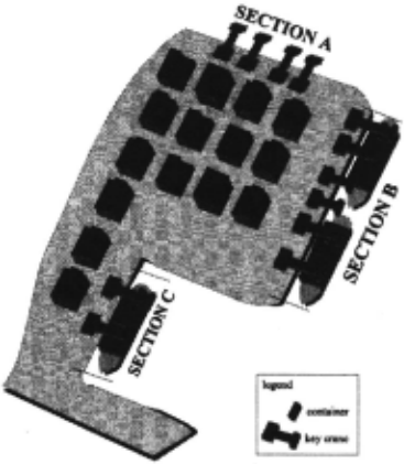
When a ship arrives at the port, the planners must first decide where to berth the ship for the unload ing and loading of containers. For the containers that are to be unloaded, the planners must decide where to place these containers in the yard. The wharf line of the port is divided into sections, and no ship can be berthed across any two sections. Which section to as sign a ship to and exactly where to berth a ship within a section depend on factors like the locations of con tainers to be loaded and unloaded, the physical (i.e. depth of the berth) and resource limitations (i.e. suit ably of quay crane) of each berth. A sketch of a port is given in Figure 1. The allocation of ships ~o sec tions and placement of containers in the yard is stud ied by Lim [Lim, 1998]. The approach used is a variant of graph partitioning problem. Allocation of vessels to sections were also studied by Brown[Brown et al., 1994; 1997].
One of the subproblems in [Lim, 1998] is the ship berthing problem. The ship berthing problem was stud ied by Heng[Heng, Khoong, and Lim, 1996] using a mixed integer linear programming model. Their model assumed constant inter-ship clearance distance and con stant end-berth clearance distance. While their model worked reasonably well on historical test data, it did quite badly on fully packed test cases. Their approach is also computationally intensive. As the ship berthing problem is only a subproblem which is called many times in the berth yard planning system, it needs to be compu tationally efficient. Heng's version of the problem is also very closely related to the offline version of the dynamic storage allocation problem [Wilson et al., 1995]. Because the dynamic storage allocation problem is a special case of the ship berthing problem, the ship berthing problem is NP-Complete [Garey and Johnson, 1979]
2 Problem Formulation
Ships come in different lengths and they arrive at the port at different times to be berthed. Every ship has an expected duration of stay which may be different from another ship. To berth a ship is to place the ship along the wharf line of a section. Once a ship is berthed, it will not be moved until its departure time. When two ships are berthed side by side, a certain minimum inter ship clearance distance must be observed. Each ship has an inter-ship clearance distance which is dependent on the ship's length. The minimum inter-ship clearance distance of two ships berthed side by side is the larger of the two ships' inter-ship clearance distances. If a ship is berthed at the end of a section, a certain end-berth clearance distance must be observed. This end-berth clearance distance is not fixed and is dependent on the ship. A ship can also be given a fixed berthing location within a section. A ship may also be prohibited from berthing at certain parts of a section. A berth plan for a set of ships in a section is the exact locations of ships within the section.
We can represent a ship geometrically by a rectangle such that the height of the rectangle is the length of the ship and the length of the rectangle is the duration of its stay. The left edge of the rectangle represents the arrival time of the ship. The right edge represents the departure time of the ship. A section can be represented geomet rically by an infinitely long rectangle where its height represents the length of the section and the length repre sents the time axis. We can associate a coordinate with the left bottom corner of the geometric representation of each ship. The z-coordinate is fixed as it represents time of arrival, but the y-coordinate is not known un less the ship has a preassigned berth location. The Ship Berthing Problem is to decide the y-coordinates of the set of boxes in the long rectangle of the section such that all rectangles representing ships are non-overlapping and are within the rectangle of the section with all clearance distances are satisfied. Figure 2 clarifies the transforma tion.
Let us define the problem formally. Let S be the set of ships {Sl,S2,····Sn}· Let bi,li,ti,di,c[,c~, and Fi be the start wharf mark of the berthing location, length, arrival time, duration of stay, inter-ship clearance dis tance, end-berth clearance distance, and the set of for bidden berth positions respectively of Ship Si. When Si is berthed at bi, Si will occupy wharf mark from bi to bi + li from time ti to time ti + di. Fi is a set of intervals in the section in which ship i cannot be berthed. If Si is berthed at bi, the interval [bi, bi + li] should not inter sect with any interval in Fi. For a clearer picture of the above definitions, please refer to Figure 2.
The optimization version of the Ship Berthing Problem The decision version of the Ship Berthing Problem is similar to the SBP problem. All we need to do is to remove the objective function to Minimize L and assume that L is given.
2.1 Complexity
Lemma 1 lf'VSi E S,li = C1,c[ = C2,c~ = Cg, where C1, C2 and C3 are constants, the ship berthing problem can be solved in 0( n log n) time.
Proof: The above problem can be transformed to the problem of coloring of interval graphs by first partition ing the section into l Li~'iJ~c, J fixed berths and sorting the ships, in non-decreasing order based on the arrival times, followed by assigning the ships in the sorted order to the fixed berths using the criteria of most recently used available berth. This algorithm takes 0( n log n) time. D
Biro[Biro et al., 1992] showed that 1-precoloring of interval graph is polynomial time solvable and 2precoloring is NP-Complete. Using his results, if '<lSi E S,li = Ct,c[ = C2,c~ = Cg, where C1,C2 and Cg are constants, and if some of the ships are preassigned to a single berth, then the problem remains polynomial time solvable. If some of the ships are preassigned to 2 berths, then the problem becomes NP-complete even if the ships have the same length and clearance distances.
In the next section, we will show the that berth planning problem is NP-complete. Our reduction uses the PARTITION problem which is known to be NP Complete. The definition of the partition problem is given below:
PARTITION Given a finite set A= {a1,a2, ... ,ax} and a size s(a) E z+ for each a E A, is there a subset A'~ A such that L:aeA' s(a) = L:aeA-A' s(a)?
Lemma 2 The berth planning problem is NP-Complete.
Proof: If we set all inter-ship clearances and end-berth clearances to be zero the berth planning problem is ex actly the same as the dynamic storage allocation prob lem [Garey and Johnson, 1979]. The dynamic storage allocation problem has been shown to be NP-complete by Stockmeyer using the 3-PARTITION problem. How ever, this result is not published[Garey and Johnson, 1979]. In this section, we shall sketch a simple reduction using the PARTITION problem. Let T = L:aeA s(a). We use the triple (li I ti I di) to represent the ship si I where li, ti, di are the length, arrival time and the du ration of stay of the ship repectively. LetS= SA USB. SA = {St, 82, Sg, ... , Sg}, where
Minimize L Subject to:
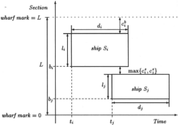
Figure 2: Geometric Representation to Graph Transformation
For the set SA, if L ~ T + 3, there are only 2 berth plans (in fact one is a reflection of the other). In both of these plans, there are two unoccuJ::>ied regions of equal size. One is from wharf mark 1 to I.+ 1, from time unit 2 to time unit 3. The other is from wharf mark I.+ 2 to T + 2 from time unit 2 to unit 3. Let SB = 1slo, Su, 0 0 0 , s9+IAI} where S; = (s(ai-9), 2, 1) . Clearly, if there is a berth plan where L ~ T + 3 then the set SB must be partitioned into two disjoint subsets such that the sum of lengths of ships in the two sub sets are the same. It is clear that the transformation will only take polynomial time. It is also clear that the problem is in NP. Hence, the berth planning problem is NP-complete. D
Since the berth planning problem is NP-Complete, it is highly unlikely that a fast algorithm can be devised to solve the problem optimally.
3 Graph Model
While the geometrical model is visually attractive, it cannot be extended to handle clearance constraints and berth restriction constraints easily. In this section, we shall transform our geometrical representation of the Ship Berthing Problem to a graph, g. For each ship S; E S, we have a vertex v; in g. The weight of vertex v; is set to l; which is the length of the ship S; . If two ships S;, Sj E S have time overlap, then there is an edge ( v;, Vj) linking the 2 vertices v; and Vj. The weight of the edge ( v;, Vj) is the larger of the two ships inter-ship clearance distances, i.e. max{ cf, cj}. For each ship S;, there are 2 additional vertices vft and vfb. These vertices have weights 0. There is a directed edge < vfb, v; > and another directed edge < v;, vft > . The weight of these directed edges is the end-berth clearance cf.
If a ship Sj is required to be fixed at a particular berth location k (i.e. bj = k and Sj will occupy wharf mark from k to k + lj) within the section, we will add two ver tices u1 and u2 and two edges< u1, Vj >and< Vj, u2 >. u1 and u2 will have vertex weight of 0. < u1, Vj > and < Vj, u2 > will have edge weight of k and L- (k + lj)· Similarly, a ship Sj may not be permitted to berth from wharf mark p to wharf mark q. We can handle this situa tion by creating a fictitious ship which is fixed at location p with length q - p - cj which has a hypothetical time overlap with only ship j . Using such a transformation, berth restrictions for ships can be handled consistently.
At the end ofthe transformation, we have a graph con sisting of directed and undirected edges. Let us pick an undirected edge e;j = ( v;, Vj). e;j exists because ship S; and ship Sj have a time overlap. This implies that both shipS; and ship Sj cannot share any part of the section. If ship S; is berthed at a lower wharf mark, (a wharf mark is a particular position in a section) than ship Sj, we will set the edge ( v;, Vj) to become < v;, Vj >. Sim ilarly, if ship Sj is berthed at a lower wharf mark than ship S;, we will set the edge e;j to go from vertex Vj to vertex v;, i.e. < Vj, v; > . The ship berthing problem has been transformed to a problem of setting the directions of undirected edges in the graph such that the graph be comes directed acyclic and the longest path in the graph is minimized. The length of a path in our graph is the sum of all vertex weights and edge weights of all vertices and edges in the path.
The directed acyclic condition of the graph is impor tant as the directions of the edges represent relative berth locations, therefore it is impossible to have a sit uation such that ship S; is berthed at a lower location than ship Sj , and ship Sj is berthed at a lower location than ship sk, and ship sk is berthed at a lower location than ship S; . Therefore, when we set the direction of the undirected edges we must not create any cycle. The length of the longest path in the directed acyclic graph created is the minimum length required in the section. to berth the set of ships S.
Lemma 3 The Ship Berthing Problem can be trans formed to a problem of fixing the directions of some edges in a graph such that the graph becomes directed acyclic and the longest path in the graph is no more than the section length.
Proof: Obvious from the above discussion.D
It is clear that the optimization version of the Ship Berthing Problem can be transformed to a problem of fixing the directions of edges in a graph such that the graph becomes directed acyclic and the longest path in the graph is minimized. In the worst case, only O(n) of the decision versions of the problem need to be solved through the use of binary search on L.
4 An Effective Greedy Algorithm
In this section, we shall discuss our heuristic for fixing the edge directions in our graph representation to create a DAG with the minimum longest path. Before describ ing the algorithm, let us define the following. Let e;j be the edge between vertices v; and Vj. If e;j is undirected, it can be set in two directions, namely from v; to Vj or from Vj to v;.
Let /3;j and /3ji be defined as follows :
Lin(v;) is the longest incoming path of vertex v;. Lout(v;) is the longest outgoing path from vertex v; . w( v;) and w( e;j) are the weights of vertex v; and edge ( i, j) respectively.
For every undirected edge, e;j, the potential of edge, cJ( e;j) is given by max{/3;j, /3j;}. The algorithm of our heuristic is given in Figure 4. The algorithm first com putes the potential of every undirected edge. Next the algorithm selects the undirected edge with the highest potential. In the event of a tie, a second criterion is used. This criterion is l/3;j - /3ji I, the larger the better. Once the edge is selected, the direction of the edge is set such that the longest path through that edge is as small as possible. In the event of a tie, the edge is set from the vertex with lower degree to the vertex with higher de gree. Next, the algorithm updates the longest incoming paths and outgoing paths, and potentials of all affected edges. This may be computed by doing 2 topological sweeps (2 passes, computing the longest incoming path for each vertex in one pass and computing the longest outgoing path for each vertex in the second pass) . A topological sweep takes O(JV(Q)I + I£(Q)I) time. Up dating will take significantly less time in practice even though the worst case time complexity stays the same. Repeat the process of finding the edge with the highest potential, fixing its direction and updating the potential of the rest of the undirected edges until the directions of all edges are set . The longest path in the graph defines the minimum section length needed. The longest incom ing path of a vertex v; defines the wharf mark whereby the ship i is to be berthed.
We shall use a simple example to illustrate our heuris tic. In our example, we assume that all clearance dis tances are zero, i.e. no clearance needed. Note that at the end of the iterations, the longest incoming path for each vertex, v; will determine the wharf mark of the ship S;.
It can be easily seen that our algorithm takes at most O{IE(Q)I(I£(Q)I + IV(Q)I) . In practice, our algorithm runs in O(JV(Q)I 2 ) time.
Lemma 4 Algorithm Greedy Berth-Planner does not create a cycle from a path.
Proof: Let us consider a cycle C = VI v2 .. . Vk -I Vk VI . Without loss of generality, let us assume that the edge eki is the last edge to fix its direction inC, which is from Vk to VI, to create the cycle C. From our graph construc tion, it is clear that the length of the path IPik I > 0 as Pik = VI v2 ... Vk. To set the edge ek I to go from Vk to VI, f3ki must be less than or equal to f3Ik (see algorithm) . This implies
From the above, it is clear that our algorithm will never turn a path to a cycle. D
Since the algorithm does not create any cycle, there will not be a situation where the algorithm is stuck, i.e. no matter which direction you fix an edge, you get a cycle. To be in such a situation, you must first have a cycle. From the above lemma, cycle detection is not needed in our heuristic.
| Algorithm Greedy Berth-Planner | |
| Step 1: | Vv; E V(Q) set Longestln(v;) = 0 and LongestOut( v;) = 0 |
| Step 2: | Ve;; E E(Q) compute cl>(e;j) |
| Step 3: | Find the undirected edge, e;;, with the highest potential cl>(e;;). If there is a tie in the highest potential; pick the edge with the largest I.B;;- ,B;;i. |
| Step 4: | If (,B;; < ,B;;) then set edge to go from v; to v; else if (,B;; > ,B;;) then set edge to go from v; to v; else if deg(v;) < deg(v;) |
| Step 5: | then set edge to go from v; to v; else set edge to go from v; to v; Update the affected longest incoming and · outgoing paths of vertices |
| Step 6: Step 7: | Update the potential of affected undirected edges If there is an undirected edge, goto 3 |
| Step 8: | |
| End | |
5 Local Search Post Optimization
Using our graph model, every arrangement is repre sented by at least an acyclic labeling. Given an acyclic labeling, the longest path and the berth position of every ship can be found in O(IV{Q)I + I£(Q)I) time. Our local search improvement approach is based on the Tabu Search method introduced by Glover [Glover, 1989; 1990]. It is applied to the solution generated by the greedy algorithm.
Given an acyclic labeling, AL, of a graph, we define the neighborhood solution of AL to be the set of acyclic labelings reachable from AL by swapping the acyclic la bels of two vertices. Among all the possible swaps, we pick the swap that improves best result seen so far. If that is not possible, we will pick the swap, that · is not forbidden by the tabu list, that returns the best result. Our tabu list's length is 10. It stores the 10 most recent swaps. The iterative improvement will be performed un til the stopping criterion is reached. The stopping cri terion is satisfied if there is no improvement of the best solution after 10 iterations or the current solution equals the lower bound.
6 Experimental Results
We have implemented our greedy heuristic and the local search algorithm in C++ using Microsoft Visual C++ development environment . We ran all our experiments on a pentium II 300MHz machine with 128 MBytes of memory. We tested our algorithms on 2 data sets and compare our algorithm with the lower bound. The lower bound is given by the maximum density. Density is given by the largest of all the sums of lengths of vessels at all points on the x (time) axis in the geometric representa tion. The first data set is the historical data from the Port. The second is manually generated. Each test case in the second data set is generated by first defining a rectangle and cutting smaller rectangles from the orig inal rectangle for each test set. In the experiments, all clearance distances are set to 0. This is to facilitate easy checking of the quality of the solutions generated. The results are summarized in Table 1 and 2.
| Historical Test Set | ||||
|---|---|---|---|---|
| Size | LB | Greedy Algorithm | Local Search PostOpt | |
| .H.esult | Ttme | |||
| 150 | 772 | 903 | 772 | 9 |
| 29 | 161 | 161 | - | - |
| 165 | 726 | 887 | 803 | 8 |
| 57 | 144 | 144 | - | - |
| 72 | 308 | 308 | - | - |
| 231 | 774 | 858 | 810 | 23 |
| 185 | 720 | 829 | 743 | 12 |
| 173 | 813 | 898 | 856 | 11 |
| 118 | 632 | 682 | 682 | 7 |
| 59 | 511 | 511 | - | - |
| 149 | 767 | 898 | 787 | 9 |
| Compact Test Set | ||||
|---|---|---|---|---|
| Size | LB | Greedy Algorithm | Local Search PostUpt | |
| .H.esult | Ttme | |||
| 15 | 20 | 20 | - | - |
| 20 | 26 | 26 | - | - |
| 30 | 25 | 32 | 25 | 2 |
| 26 | 24 | 29 | 24 | 1 |
| 40 | 25 | 29 | 27 | 6 |
| 50 | 20 | 25 | 22 | 10 |
| 100 | 20 | 26 | 23 | 19 |
The first column of the tables is the number of ships. The second is the density. The third is the result ob tained by the greedy method. The greedy took less than 1 seconds for all the test cases in our experiment. The fourth and fifth columns are the result and time taken in seconds respectively by the local search algorithm.
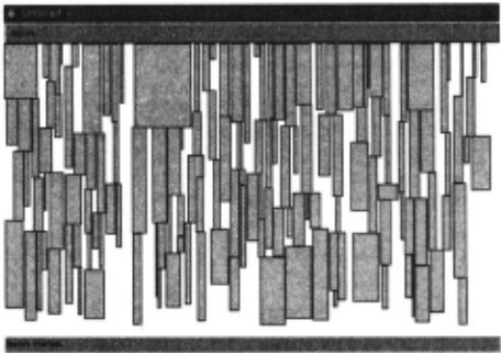
A sample solution of a test case is given in Figure 5.
7 Conclusion
In this paper, we formulated the ship berthing prob lem, analyzed its complexity and transformed the geo metric version of the problem into a graph proplem. We also proposed a fast and effective greedy algorithm which when used with a tabu search like post optimization rou tine can return optimal or near optimal solutions.
8 Acknowledgment
This research was motivated by a project the first au thor had with the Port of Singapore Authority. This research was supported in part by the NUS Research Grant RP3972679.
@inproceedings{ijcai1999p85,
  title     = {An Effective Ship Berthing Algorithm},
  author    = {Lim, Andrew},
  booktitle = {Proceedings of the Sixteenth International Joint Conference on
               Artificial Intelligence, {IJCAI-99}},
  publisher = {International Joint Conferences on Artificial Intelligence},
  editor    = {Thomas Dean},
  pages     = {594--598},
  year      = {1999},
  note      = {Knowledge-based Applications},
  url       = {https://ijcai.org/proceedings/1999/85},
}
TY - CPAPER TI - An Effective Ship Berthing Algorithm AU - Lim, Andrew T2 - Proceedings of the Sixteenth International Joint Conference on Artificial Intelligence, IJCAI-99 PB - International Joint Conferences on Artificial Intelligence PY - 1999 SP - 594 EP - 598 UR - https://ijcai.org/proceedings/1999/85 ER -Copied
Machine-readable versions of this paper, for tools and AI agents:





