Algorithms for Optimizing Leveled Commitment Contracts

1 Introduction

In multiagent systems consisting of self-interested agents, contracts have traditionally been binding [Rosen­ schein and Zlotkin, 1994; Sandholm, 1993; Kraus, 1993] . Once an agent agrees to a contract , she has to follow through no matter how future events unravel. Although a contract may be profitable to an agent when viewed ex ante it need not be profitable when viewed after some futu;e events have occurred, i.e. ex post. Similarly, a contract may have too low expected payoff ex ante, but in some realizations of the future events, it may be de­ sirable when viewed ex post. Normal full commitment contracts are unable to take advantage of the possibili­ ties that such future events provide.

On the other hand, many multiagent systems consist­ ing of cooperative agents incorporate some form of de­ commitment in order to allow agents to accommodate new events. For example, in the original Contract Net Protocol [Smith, 1980], the agent that contracts out a task could send a termination message to cancel the contract even when the contractee had partially fulfilled it. This was possible because the agents were not self­ interested: the contractee did not mind losing part of its effort without a monetary compensation. Similarly, the role of decommitment among cooperative a~ents has been studied in meeting scheduling [Sen, 1993j.

*This material is based upon work supported by the National Science Foundation under CAREER Award IRI-9703122, Grant IRI-9610122, and Grant IIS-9800994.

Contingency contracts have been suggested for utiliz­ ing the potential provided by future events among ~elf­ interested agents [Raiffa, 1982]. The contract obliga­ tions are made contingent on future events. In some games this increases the expected payoff to both parties compared to any full commitment contract. However, contingency contracts are often impractical because the space of combinations of future events may be large and unknown. Also, when events are not mutually observ­ able, the observing agent can lie about what transpired.

Leveled commitment contracts are another method for capitalizing on future events [Sandholm and Lesser, 1996]. Instead of conditioning the contract on future events a mechanism is built into the contract that allows unilat~ral decommitting. This is achieved by specifying in the contract the level of commitment by decommit­ ment penalties, one for each agent. 1 If an agent wants to decommit-i.e. to be freed from the obligations of the contract-it can do so simply by paying the decommit­ ment penalty to the other party. The method requires no explicit conditioning on future events: each agen~ can. do her own conditioning dynamically. No event venficatwn mechanism against lying is required either.

Principles for assessing decommitment penalties have been studied in law [Calamari and Perillo, 1977; Pos­ ner, 1977], but the purpose has been to assess a penalty on the agent that has breached the contract after t_he breach has occurred. Similarly, penalty clauses for parttal failure- such as not meeting a deadline-are commonly used in contracts, but the purpose is usually to. moti­ vate the agents to follow the contract. Instead, m lev­ eled commitment contracts, explicitly allowing decom­ mitment from the contract for a predetermined price is used as an active method for utilizing the potential pro­ vided by an uncertain future. 2 The decommitment pos­ sibility increases each agent's expected payoff under very general assumptions [Sandholm and Lesser, 1996] .

I [Sandholm and Lesser, 1995] present an example protocol that uses this feature .

2Decommitting has been studied in other settings, e.g. where

We analyze contracting situations from the perspec­ tive of two risk neutral agents each of which attempts to maximize his own expected payoff: the contractor who pays to get a task done, and the contractee who gets paid for handling the task. Handling a task can mean taking on any types of constraints. The method is not specific to classical task allocation. The contractor tries to minimize the contract price p that he has to pay. The contractee tries to maximize the payoff p that she re­ ceives.

We study a setting where the future of the agents in­ volves uncertainty. Specifically, the agents might receive outside offers. 3 The contractor's best outside offer a is only probabilistically known ex ante by both agents, and is characterized by a probability density function f (a) . If the contractor does not receive an outside offer, a cor­ responds to its best outstanding outside offer or its fall­ back payoff, i.e. payoff that it receives if no contract is made. The contractee's best outside offer b is also only probabilistically known ex ante, and is characterized by a probability density function g(b) . If the contractee does not receive an outside offer, b corresponds to its best outstanding outside offer or its fall-back payoff. 4 The variables a and b are assumed statistically independent.

The contractor's options are either to make a contract with the contractee or to wait for a. Similarly, the con­ tractee's options are either to make a contract with the contractor or to wait for b. The two agents could make a full commitment contract at some price. Alternatively, they can make a leveled commitment contract which is specified by the contract price, p, the contractor's decom­ mitment penalty, a, and the contractee's decommitment penalty, b. We restrict our attention to contracts where a 2: 0 and b 2: 0, i.e. agents do not get paid for decom­ mitting. The contractor has to decide on decommitting when he knows his outside offer a but does not know the contractee's outside offer b. Similarly, the contractee has to decide on decommitting when she knows her out­ side offer b but does not know the contractor's. This seems realistic from a practical automated contracting perspective.

The theory of these leveled commitment protocols was presented by [Sandholm and Lesser, 1996], but to date no algorithms have been presented for agents to com­ pute when they should decommit given a contract, or for agents to choose beneficial contracts. This paper oper­ ationalizes leveled commitment contracts by presenting an algorithm for computing how the agents should decommit (Section 2), and an algorithm for constructing the optimal leveled commitment contract for any given setting defined by f(a) and g(b) (Section 3) .

there is a constant inflow of agents , and they have a time cost for searching partners of two types: good or bad [Diamond and Maskin, 1979].

3 The framework can also be interpreted to model situations where the agents' cost structures for handling tasks and for get­ ting tasks handled change e.g. due to resources going off-line or becoming back on-line.

4 Games where at least one agent's future is certain, are a subset of these games. In such games all of the probability mass of f(a) and/or g(~) is on one point .

2 Nash equilibria for a given contract

One concern is that a rational agent is reluctant in de­ committing because there is a chance that the other party will decommit , in which case the former agent gets freed from the contract , does not have to pay a penalty, and collects a penalty from the breacher . [Sandholm and Lesser, 1996] showed that despite such insincere decom­ mitting the leveled commitment feature increases each contract party's expected payoff, and enables contracts in settings where no full commitment contract is bene­ ficial to all parties. To set the context, we first review their analysis of how rational agents would decommit , i.e. we derive the Nash equilibrium (NE) [Nash, 1950] of the decommitting game where each agent 's decom­ mitting strategy is a best response to the other agent 's decommitting strategy. The new contributions begin in Section 2.3.

The contractor decommits if he gets a low enough out­ side offer, e.g., he can get his task handled at a low cost . We denote his decommitting threshold by a* , so his de­ committing probability is

The contractee decommits if she gets a high enough outside offer, e.g., gets paid for handling a task. We denote her decommitting threshold by b* , so her decom­ mitting probability is

2.1 Sequential decommitting (SEQD) game

In our sequential decommitting (SEQD) game, one agent has to reveal her decommitting decision before knowing whether the other party decommits. While our imple­ mentation analyzes both orders of decommitting, due to space limitations we only discuss the setting where the contractee has to decide first . The case where the contractor decides first is analogous. There are two al­ ternative leveled commitment contracts that differ on whether or not the agents have to pay the penalties if both decommit.

If the contractee has decommitted, the contractor 's best move is not to decommit because -a-a+b::; -a+b (because a 2: 0) . This also holds for a contract where neither agent has to pay a decommitment penalty if both decommit since -a ::; -a+ b. In the subgame where the contractee has not decommitted, the contractor's best move is to decommit if -a- a > -p, i.e.

The contractee gets b - b if she decommits , b + a if she does not but the contractor does, and p if neither decommits. Thus the contractee decommits if b - b > Pa(b +a)+ (1- Pa)p. If Pa = 1, this is equivalent to -b > a which is false because a > 0 and b > 0. In other words, if the contractee surely deZommits, the contractor does not . On the other hand, the above is equivalent to

(4a)

2.2 Simultaneous decommitting games

In our simultaneous decommitting games, agents have to reveal their decommitment decisions simultaneously. We first discuss the variant (SIMUDBP) where both have to pay the penalties if both decommit . The contractor decommits if Pb · (-a+ b- a)+ (1- Pb)(-a- a) > Pb ·(-a+ b)+ (1- Pb)(-p). If Pb = 1, this equates to a < 0, but we already ruled out contracts where an agent gets paid for decommitting. On the other hand, this equates to

The contractee decommits if (1- Pa)(b- b)+ Pa(b­ b +a) > (1- Pa)P + Pa(b +a). If Pa = 1, this equates to b < 0, but we ruled out contracts where an agent gets paid for decommitting. However, this equates to

In a SIMUDNP game, neither agent has to pay if both decommit. The contractor decommits if Pb · (-a)+ (1Pb)(-a- a)> Pb ·(-a+ b)+ (1- Pb)(-p) . If Pb = 1, this equates to b < 0, but we already ruled out contracts where an agent gets paid for decommitting. On the other hand, this equates to

The contractee decommits if (1- Pa)(b- b)+ Pab > (1- Pa)P + Pa(b +a). If Pa = 1, this equates to a < 0, but we ruled out contracts where an agent gets paid for decommitting. However, this equates to

For each game, calculating the Nash equilibria amounts to solving the simultaneous equations (3) and (4) which use (1) and (2).

2.3 Existence of a Nash equilibrium

We now discuss existence of the NE. Denote the support of f(a) by [a1, an], and the support of g(b) by [b1, bm] ·

Proposition 2.1

SEQD: A NE exists if a1 ~ p- a~ an. NoNE exists if p - a > an . Only a trivial NE with Pa = 0 exists if p- a< al.

SIMUDBP: A NE exists if p- a 2: an and p + b ~ b1 . Only a trivial NE with Pa = 0 exists if p - a < a1 and p + b > b1 . Only a trivial NE with Pb = 0 exists if p+b > bm and p-a <an. Otherwise a NE may or may not exist.

SIMUDNP: A NE exists if p- a 2: an and p + b 2: bm. Only a trivial NE with Pa = 0 exists if p- a .< a1 and p + b > b1. Only a trivial NE with Pa = 0 and Pb = 0 exists if p- a < a1 and p + b > bm. No NE exists if p + b < b1 . Otherwise a NE may or may not exist.

Proof. For each of the three games, the curves defined by (3) and (4) are continuous.

SEQD: From (3a): a· = p- a. For (4a), when a· = a1, b* = p + b and in the limit a· -+ an, b* -+ oo. Thus the curves intersect if a 1 ~ p - a ~ an . For ( 4a) if p- a < al then b* = p + b, and so (3a) intersects with ( 4a) such that Pa = 0. For p- a > an (3a) and ( 4a) do not intersect.

SIMUDBP: For (3b), in the limit b* -+ b1, a* -+ -oo and when b* = bm , a* = p- a. For (4b) , when a· = a1, b* = p + b and in the limit a· -+ an, b* -+ oo. Thus the curves intersect if p- a 2: an and p + b ~ b1 For ( 4b) if a· < al then b* = p + b, and so the two curves will intersect with Pa = 0 if p + b > b1 . Similarly for (3b) if b* > bm then a· = p - a, and so the two curves will intersect with Pb = 0 if p - a < an . Otherwise they may or may not intersect.

SIMUDNP: For (3c), in the limitb*-+ b1, a*-+ -oo and when b* = bm, a· = p- a. For (4c), when a* = a1, b* = p + b and in the limit a· -+ an , b* -+ - oo. Thus the curves intersect if p - a 2: an and p + b 2: bm . For ( 4c) if a· < ill then b* = p + b, and so the two curves intersect with Pa = 0 if p + b > b1 . Further if p + b > bm then Pb also equals 0. The curves do not intersect if p + b ~ b1. Otherwise they may or may not intersect . 0

2.4 Uniqueness of the Nash equilibrium

We now consider uniqueness of the Nash equilibrium.

Proposition 2.2 For the sequential games, the NE is umque. For the simultaneous games the NE need not be umque.

Proof. For the sequential games, uniqueness follows from the forms of (3) and ( 4) : One threshold is expressed as a function of p and a penalty, and the other is defined as a function of this threshold. Fig. 1 shows an example where multiple equilibria exist for a SIMUDBP game. We constructed a similar example for SIMUDNP. 0

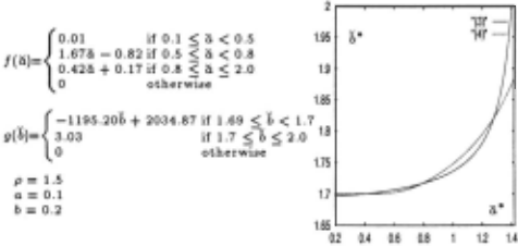
2.5 Algorithm for finding the Nash equilibria We now discuss the algorithm for computing the Nash equilibria. We assume that the probability density func­ tions f(a) and g(b) are piecewise linear with n and m pieces respectively. This is reasonable since any continu­ ous function can be approximated arbitrarily closely by a piecewise linear curve, and piecewise linear curves are easy for the user to input.

The algorithm for computing the equilibrium of a se­ quential game is straightforward. It simply substitutes the contract parameters (p, a, b) into (3) and ( 4) .

In the simultaneous games this substitution gives a system of two nonlinear simultaneous equations. These equations may have multiple solutions and all of them need to be found. This rules out iterative procedures that only find one solution. That motivated us to design a fast analytic algorithm that finds all solutions. We decompose the search space into rectangles. Since f(a) and g(b) are piecewise linear, the simultaneous equations can be solved analytically within each rectangle. The rectangles are [a;, a;+l] x [bj, bj+l] where 1 ~ i <nand 1 ~ j < m, i.e. the boundaries are the end points of each linear segment of f and g. Within each rectangle, the algorithm

1. Solves (1) and (2) to get Pa(a*) and Pb(b*). These functions are quadratic because f(a) and g(b) are linear within the rectangle.
2. Substitutes Pa(a*) into (4), and Pb(b*) into (3).
3. Substitutes a· from (3) into ( 4).
4. Reduces the resulting equation to a cubic polynomial in b*.
5. Solves for the roots of this polynomial.
6. Calculates the corresponding values for a· using (3).
7. Accepts the solutions that lie within the rectangle.

The algorithm runs in O(nm) time because it is 0(1) within each rectangle, and there are O(nm) rectangles.

Of all the equilibria found, it presents social welfare maximizing one( s) to the user, i.e. the one( s) that maxi­ mize the sum of the agents' expected payoffs. It can also present all equilibria.

3 Optimizing the contract

So far we discussed how rational agents would decommit under a given contract. Now we take this further by optimizing the contract itself-taking into account that agents will decommit insincerely in Nash equilibrium. Specifically, we present an algorithm and analysis for finding the optimal contract price and decommitment penalties in any given setting for all three protocols.

3.1 Analysis

We first describe the optimization problem. Let 7ra be the contractor's expected utility, and 7rb the contractee's. For shorthand, we define T1 , T2, T3, and T4:

We now derive 7ra and 7rb for each of the games.

SEQD:

SIMUDBP:

SIMUDNP:

For each of the three protocols the social welfare, ;rr, is

We define the optimal contract to be the contract that maximizes social welfare, i.e. max(p,a,b)1r· The expres­ sion above shows that 1r is the same for all three games. Also, 1r is a function of ( a·, b*). So, the original problem of optimizing over a 3-dimensional space (p, a, b) reduces to optimizing over a 2-dimensional space ( a·' [;·).

A rational agent only accepts a contract if it does not decrease his expected payoff. These individual rational­ ity (IR) constraints, 1r a 2:: E[ -a] and 7rb 2:: E[b], define a feasible set in the 3-dimensional space ( a·' b*' p) .

We first derive the unconstrained optima, and then verify that they belong to the feasible set . The necessary conditions for unconstrained optima are: 5

These equalities are trivially satisfied if f( a·) = 0 or g(b*) = 0, i.e. if the optimal decommitting thresholds occur in a gap in f or g. In such cases, there necessarily is another pair of optimal thresholds where the old optimal threshold that was in the gap is now at the end of the gap. This is because the probability mass in the gap is zero so moving a decommitting threshold to the end of the gap cannot affect the path of play. Therefore, we can restrict our analysis to the case where f(a*) > 0 and g(b*) > 0.

5 In deriving the formulas on the right, the derivative of an integral with respect to its limits is calculated using the Leibnitz formula [Arfken and Weber, 1995].

The first order constraints above are satisfied if E[b]­ T4 - a· + a*Ta = 0 and b*T1 - T2 = 0. These two conditions give a pair of simultaneous equations:

Equation (5) describes a· as a function of b* and Equa­ tion (6) gives b* as a function of a·. A local optimum of 1r exists where the curves intersect . They may or may not intersect, and they can intersect at multiple points:

Proposition 3.1 Curves (5) and (6) intersect if E[a] 2: b1 and E[b] :S an . They do not intersect if b1 > an. Oth­ erwise they may or may not intersect. The intersection point is unique if bm < E[a] or a1 > E[b].

Proof. From (5), in the limit b* -+ b1 , a· -+ b1 and when b* 2: bm, a· = E[b]. From (6), when a· :S a1 , b* = E[aJ and in the limit a· -+ an, b* -+ an. Both curves represent strictly increasing functions (the first derivatives are always positive). Note that T1 =f:. 1 => b* > b1, and Ta =f:. 0 => a* < an. Thus they intersect if E[a] 2: b1 and E[b] :S an. This intersection point is unique if bm < E[a] or a1 > E[b]. They do not intersect if b1 >an. Otherwise they may or may not intersect. D

Figure 2 shows that (5) and (6) can intersect at multi­ ple points, i.e. that 1r can have multiple (local) optima.

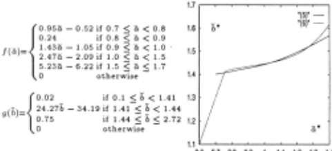
0.6 0.7 0.8 0.9 1 1.1 1.2 1.3 1.4

Figure 2: Example with 3 local optima.

We now show that if these locally optimal solutions exist, they lie within the feasible set, i.e. there exists a nonempty range [LB, U B] for the contract price p which satisfies the IR constraints. We derive LB and U B using the expressions for 7ra, 7rb and the IR constraints, 7ra 2: - E[a], 7rb 2: E[b], to get:

SEQD:

SIMUDBP: LB- b'T3Tt+ii'(1-Tt)(1-T3)+E[b]T3-T3T2 - 1 T,+T3Tt U B = b'T3Tt+li'(1-T1 )(1-T3 )+T4 (1-Tt)

SIMUDNP:

1-T,+T3Tt

For SIMUDBP games, 1-T1 +T3T1 =f:. 0. For SIMUDNP, (1 - Tt)Ta =f:. 0. This occurs from the form of the in­ tegrals, and the fact that they are always between 0 and 1 because they are defined over probability density functions. For each game above, LB :::; U B reduces to T (E[b] - T) < T. (1 - T) <:::> E[I>]-T 2 < 'b _....... a* < b* 3 2 - 4 1 1-T 1 - T3 -...,. - which can be shown true by the form of (5) and (6) .

3.2 Algorithm for finding optimal contracts

Our algorithm determines the optima by computing the intersection points of curves (5) and (6) . Multiple so­ lutions might exist, which rules out the use of iterative methods that only find one solution. Our algorithm uses the same rectangular decomposition as our equilibrium finding algorithm presented above. In each rectangle it

1. Solves T1,T2,Ta, and T4 to get quadratic equations for them (because f(a) and g(b) are linear within the rectangle).
2. Substitutes these into (5) and (6).
3. Substitutes a· from (5) into (6).
4. Reduces the resulting equation to a 9th degree polynomial in b*.
5. Solves for the roots of this polynomial.
6. Calculates the corresponding values of a· from (5).
7. Accepts solutions (a*, b*) that lie in the rectangle. The algorithm runs in O(nm) time because it is 0(1) within each rectangle, and there are O(nm) rectangles. Finally, the candidate set of local optima is scanned for global optima.

3.3 The fair optimal contract

An optimal pair (a*, b*) defines a set of welfare max­ imizing contracts (p, a, b) which differ based on how the excess-i.e. expected gain over full commitment contracts-is divided among the contract parties. Our implementation shows all the optimal feasible contracts to the user and visualizes how the different choices lead to different division of expected payoff ( 1r a and 7rb as lin­ ear functions of p E [ LB, U B]). It also suggests a fair contract which divides the excess e~ual~. It turns out that the fair contract price is p = ~. The fair val­ ues for the penalties are then calculated using (3) and ( 4).

4 Implementation

Using the algorithms of this paper, we provide a client­ server based contract optimizing service on the web (http://ecommerce.cs.wustl.edu/contracts.htrnl) as part of eMediator, our next generation electronic com­ merce server. The client, a Java applet , implements the GUI and communicates to the server over the web using CGI/Perl. The server, written in C, executes the com­ putations. The client accepts piecewise linear functions f(a) and g(b). The user can input these graphically or as text . Each probability density functions is automatically scaled so that its integral is 1. The output interface dis­ plays either the decommitting thresholds and probabili­ ties for a given contract, or the optimal feasible contracts together with the fair optimal feasible contract.

The server computes the roots of polynomials in our rectangular decomposition algorithms. We use Laguer's root finding method to compute the roots [Press et al., 1993) . It finds all roots simultaneously and polishes roots to reduce numerical imprecision. If the roots are close to the boundaries of the rectangle, imprecision may result in these roots being calculated just outside the rectangle. To accommodate for this, we extend the rectangle in all directions by f. That allows us to capture all those roots that would otherwise be overlooked.

5 Generalization to 3-agent contracts

The method can be generalized to contracts involving more than two agents. We demonstrate this via 3-agent games. Let there be one contractor, a, and two con­ tractees, b and c. If even one party decommits the con­ tract breaks down between all 3 parties. Let the density functions of outside offers be f(a), g(b), and h(c). The IR constraints are rr a 2:: E[ -a], 7rb 2:: E[b], and rr c 2:: E[C] . The contract price, p, paid by the contractor, is paid in two parts, p1 to b, and p- p1 to c. The decommitment penalties are ab,ac,ba,bc,ca, and Cb, see Figure 3.

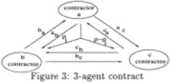
The sequential game will have 3! variants depending on the decommitting order. The simultaneous games differ based on whether two parties on simultaneous de­ commitment pay each other or not. Due to limited space we only present the formulae for SIMUDBP:

These expressions are analogous to 2-agent SIMUDBP. We get similar expressions for 1l"a, 7rb, 1l"c,and rr. Our rectangular decomposition algorithms for computing the Nash equilibria extend by using cuboids instead of rect­ angles. Nonuniqueness extends to this case. The opti­ mization problem also has similar characteristics. 1r is a function of a· , b*, c·. Solving for the roots of the first derivatives yields three equations in three variables. Our rectangular decomposition algorithms for calculating the optima extend to this case by using cuboids instead of rectangles. Similar expressions/results occur for the 3agent generalization of SIMUDNP.

6 Conclusions

Leveled commitment contract are a practical way of cap­ italizing on future uncertainties in negotiation among self-interested agents. This paper operationalizes them by presenting two algorithms . The first one takes a given contract and computes the Nash equilibrium decommit­ ting thresholds and decommitting probabilities for ra­ tional agents. The second algorithm optimizes the con­ tract price and penalties so as to maximize the sum of the agents' expected payoffs -taking into account that agents decommit insincerely. Using these algorithms, a contract optimizing service is provided on the web.