Computing Near Optimal Strategies for Stochastic Investment Planning Problems

1 Introduction

Investment is an act of incurring immediate cost in the ex­ pectation of future rewards. Investments options are typi­ cally characterized by three parameters: the initial and ac­ cumulated costs, the uncertainty over the future rewards, and the leeway in timing the actions. Investors try to optimize their decision with respect to these parameters. Modern eco­ nomics theory models the uncertainty of future rewards as a stochastic process defining future price curves. The pro­ cess is typically an Ito process [Dixit and Pindyck, 1994] that is Markovian, thus investment decision can be modeled as a Markov decision process (MDP) where a state of the un­ derlying process needs only to include the current investment portfolio and current prices. While the MDP gives a succinct formalization of the investment decision processes it does not necessarily imply efficient algorithms for computing optimal strategies. The Markov decision process has a continuous state space and a potentially large action space and cannot be solved efficiently by standard dynamic programming meth­ ods. A challenging goal in this research area is to character­ ize special cases of the general investment paradigm that are interesting enough from the application point of view while simple enough to allow efficiently computable analytic solu­ tions.

In this work we focus on stochastic planning in the context of commodity trading. Commodity can be bought, stored and eventually sold. In addition to the initial cost of buying the commodity, the investment decision must take into account the accumulated cost of storage till the commodity is sold. A standard assumption in mathematical economics is that com­ modity prices (e.g oil and copper) are best modeled as a mean reverting stochastic process. We study several versions of the commodity trading problem. In the simplest version we as­ sume that there are no restrictions on the amount of commod­ ity that an investor can buy, store or sell at a given time. We give an efficiently computable optimal analytic solution for that case. The problem becomes significantly harder when we turn to a more realistic setting in which there are constrains on the amount of commodity that a trader can buy store and in particular sell at a given time. We present an efficient Monte­ Carlo technique that generates an approximate optimal trad­ ing policy with volume and storage constrains.

1 Supported by a research grant from Goldman Sachs.

2 Supported in part by NSF grant CCR- 9731477.

There has been extensive research in AI in recent years on solving MDPs with large state spaces exploiting specific problem structures, in particular through factoring and de­ compositions [Boutilier et al., 1995; Dearden and Boutilier, 1997; Dean and Lin, 1995; Meuleau et al., 1998]. How­ ever all these work assume finite or at least discrete state spa~e . Our solution relies on structure analysis of the problem combined with a Monte-Carlo approximation technique. We show that when prices follow a mean-reverting process, the optimal policy for the constrained commodity trading prob­ lem has an elegant compact parametric form. This observa­ tion allows for a significant reduction in the space of possible optimal policies. Furthermore, we show that individual pa­ rameters, which represent a stack of decision thresholds, can be optimized incrementally thus further reducing the com­ plexity of the problem-solving task.

2 The Model

Mathematical economics models commodity price fluctua­ tions as an Ito mean-reverting process (Ornstein-Uhlenbeck process) [Dixit and Pindyck, 1994], where changes in price p satisfy a stochastic differential equation

such that dz is the (random) increment of a Wiener process (Brownian motion with normally distributed increments), J.l is the long term average price of the commodity i.e. a value to which the process reverts, TJ is the speed of reversion, and cr is the standard deviation of the random component.

Trading occurs at discrete time steps, and price fluctuation between two consecutive steps is modeled by the discrete ver­ sion of the mean-reverting process [Dixit and Pindyck, 1994]:

where ft is a sequence of independent random variables with normal distribution N(O, a-f), a-; = ~~ (1- e- 2 '7).

The agent (investor) can buy and sell the commodity at dif­ ferent time steps. There is a fixed cost q for storing a unit of community for a unit time interval. The cost of money (the interest rate) is denoted by r. We assume that the volume of commodity traded by the agent is small with respect to the to­ tal market of that commodity, so that the agent's strategy does not affect the above parameters. In the more general setting there are limits on the number of units a trader can buy and sell in every step, and on the total number of units that can be stored (denoted Cbuy· Gsell · Cstore respectively).

Objectives

Our goal is to determine the best, profit maximizing, trading strategy for a given initial state, which is determined by the current price and amount of commodity the agent owns. We use the standard valuation method, the expected net present value (NPV) function (see e.g. [Brealey and Myers, 1991; Trigeorgis, 1996])):

where s denotes an initial state, 1r is a strategy, 1 = 1 !r is a discount factor, Tis the decision horizon, and mt is cash flow at timet. Thus our goal is to find 1r such that V ,. ( s) is maxi­ mized. The objective function corresponds to discounted ver­ sions of standard finite or infinite horizon criteria (see [Bell­ man, 1957; Puterman, 1994]) where rewards correspond to cash flows.

In the following we focus on the infinite horizon invest­ ment problem. The trading strategy for this case is repre­ sented as 1r : R x N -+ N mapping the current price Pt and number of units of commodity we own- Ct to the number of units to be held in the next step - Ct+l · The results for the infinite trading horizon can be adopted to the finite horizon problem.

Example

Our model fits a variety of applications. A typical example is oil-trading problem. Oil can be bought and sold in the market. The changes of oil prices on the market follow the mean reverting process [Dixit and Pindyck, 1994] and indi­ vidual trading activities do not affect the market price. Oil can be stored at a fixed cost per unit, and there are obvious constraints on the amounts that can be stored and released in short time intervals.

3 Standard approach and its shortcomings

The value (expected NPV) of a strategy 1r can be expressed using the Bellman equation [Bellman, 1957]:

where a state is a cross-product of a commodity price p and the amount of commodity held c; R(p, c, 1r(p, c)) denotes the expected one-step cash flow resulting from action 1r(p, c); r maps the current commodity holdings to the next state com­ modity holdings under the action dictated by the policy 1r; and f(p'lp) denotes a distribution of next state prices p' (a normal distribution defined by Equation 1 ). In general it is extremely hard to evaluate a given strategy because of the size of a state space we face (in one step we can reach any price) and there is no closed form solution to the integral part. The task of finding the optimal policy is even worse as the space of poli­ cies we need to choose from is even larger. Thus, standard dynamic programming approaches cannot be applied directly and we must resort to methods that exploit the problem struc­ ture.

4 Trading without constraints

To solve the case with no limits on buy, sell and store activi­ ties, it is sufficient to study the problem of investing one unit of commodity, since the strategy for one unit can be replicated for any number of units.

A strategy for the one-unit problem at any point in time is restricted to only two choices: 0 (do not invest, do not hold the commodity) and 1 (hold, invest in the commodity). Because buy and sell prices are always the same and prices change independently of our trading, the expected net present value of a one-unit strategy 1r (V,.) can be expressed in terms of step-wise gains:

where Yt = -Pt - q + / Pt+l is the gain from time step t, q is a fixed storage cost, holdt = 1 if the strategy 1r chooses to hold the commodity at time t and holdt = 0 when not.

Intuitively, we can replicate payoffs from any strategy by always selling the commodity held at the end of the step and buy it back when the strategy requires us to hold the com­ modity in the next time step. The term p0c0 reflects the fact that we always sell (pretend to sell) the initial commodity at price p0 . Thus, we can restrict our search to policies of the form 1r : R-+ {0, 1} , mapping prices to actions. The value function for such a policy 1r can be rewritten as:

where vrr (po , 0) is the value function for the policy 7r starting from a zero commodity state. vrr (p, 0) satisfies

E(g1 (p) ) is the expected gain for holding the commodity for one step starting from price p

p' denotes the next step price, q 2: 0 is a storage cost and E(p'lp) is the expected next step price. A nice feature of Equation 2 is that the contribution from following the policy 1r in the future (integral part) is independent of the action choice in the first step. This leads to the fact that the greedy one-step lookahead strategy is optima1. 1

Theorem 1 The strategy 11' maximizing the expected one-step gain is optimal.

Proof Follows directly from Equation 2 and the indepen­ dence of future values on current actions. D

The value of the optimal one-unit policy can be written as:

with E(g0 (p)) = 0 denoting the expected gain for holding zero units of commodity. The optimal policy satisfies:

The important thing about this is that we know how to find the optimal policy easily and this despite the fact that its value is hard to compute.

4.1 Decision threshold

As the expected gain from not holding the commodity is 0, the choice to hold the commodity is justified only when E(gl(p)) 2: 0, that is, when the expected gain is positive. Substituting p' using equation 1, we get the condition for choosing the "hold" action:

Thus, we obtain a simple and compact policy: Hold the com­ modity when the price pis lower than Pi· Note that the op­ timal threshold price Pi depends solely on the parameters of the mean reverting process and discount I·

5 Trading with constraints

We consider three types of constraints: buy, sell and store limits. We start with buy and store constraints.

5.1 Buy and store constraints

The buy and store constraints are relatively easy to handle when no restriction on the sell is imposed. Simply, we al­ ways want to take the maximum advantage of a positive gain for investing in the next step. Thus, we always hold the max­ imum amount of commodity allowed by the buy and store limits, whenever the optimal one-unit policy recommends to hold. That is:

Cbuy and Cstore denote buy and store constraints.

1 We note the optimality of a greedy one step lookahead strategy holds not only for the mean reverting process, but also for a more general Ito process.

5.2 Sell limit problem

The sell limit is tricky, since a trader may not be able to im­ mediately realize all gains if he holds more units than the sell limit. A naive solution would be to limit the holding to the sell limit, but such policy is obviously sub-optimal.

In studying this case we can assume w.l.o.g. that the sell limit is 1. The solution for an arbitrary sell constraint Gsell 2: 1 is then obtained by replicating the optimal strategy with sell limit 1. In the following we first study a special case in which a trader is allowed to hold at most 2 units of commodity (with sell constraint 1) and find the corresponding optimal policy. Later we generalize the idea to any number of units.

5.3 Trading two units under sell limit

To solve the two units case we restrict our attention to strate­ gies that always try to trade the first unit using the optimal one-unit strategy. Then our goal is to simply find how and when to invest in the second commodity. We show later that this approach indeed leads to the optimal solution.

Let ll2 be a set of policies 7r2 : R -t { 0, 1, 2} mapping cur­ rent prices to commodity choices, such that 7r2 always follows the optimal one-unit strategy for the first unit and chooses to hold the second unit arbitrarily but only when p :=:; Pi . Thus 1i"2 is described as:

Note that a strategy 7r2 E ll2 may not be directly appli­ cable to the two-unit case and can violate the sell capacity. This happens when 7r2 recommends to hold two units of the commodity for some price p :=:; Pi in one step and is forced to recommend 0 units when the next step price p' jumps above

Pi· To fix this problem we define a set of policies TI2, such that for every 7r2 E ll2 there is a policy 11'2 : R x { 0, 1, 2} -t {0, 1, 2} in TI2, mapping current price and current commodity holding to the next step commodity choice and is defined as:

The idea behind 11'2 is that it replicates 7r2 when it is consistent with sell constraints, otherwise it recommends to reduce the number of units of commodity held by 1. Because 7r2 induces 11'2 we call it a generating policy.

To find the optimal investment rule for the second unit we trf to quantify its added value. To do this, we create a strategy 11'2 that recommends to hold two units of commodity when p ::; Pi and this only for the first step, otherwise it follows the optimal one-unit policy. The value for such a policy for price p ::; Pi, and zero units of commodity in terms of gains is:

Note that due to the sell limit the second unit of commodity is always held also in the second step. This is captured by the term E(g1 (p') ). The key trick now is to rewrite V"; (p, 0) for p::; Pi as:

where

is the expected added gain for investing in the second unit of commodity for p :S Pi. E(g2 (p)) represents the difference from investing in the second unit of commodity at p :S Pi compared to the optimal one-unit strategy. It consists of two terms: the expected gain from holding the commodity for one step plus a correction term (a kind of expected loss or negative gain) for holding it one more step in the case we would like to sell it (p' ;::=: pi), but sell constraint does not allow us to do that. Note that E(g2 (p)) depends solely on the price of a commodity and also E(g2(p)) :S E(gl(P)).

The other important feature is that by substituting Vt (p, 0) from Equation 3, the value V1r; (p, 0) for p :S Pi equals:

which means that the integral part of the expression now be­ comes independent of the commodity held in the first step and disregards any units we were not able to sell. Intuitively, un­ der expectations, the term E(g2 (p)) allows us to pretend that we were able to sell both units at the end of the previous step without restriction, though in reality when the price p' climbs above Pi we have to keep one unit and sell it later when the sell capacity is available.

Using the fact that E(g2 (p)) allows us to disregard any commodity left from previous steps we can express the value function for an arbitrary policy rr2 E I12 as

For zero units of commodity the policy rr2 always equals its generating 1r2 (see equation 5) and therefore

This means that if we want to find the optimal rr2 from I12 we can do it by simply finding the optimal1r2 from ll2.

Theorem 2 The optimal two-unit strategy rri E I12 max­ imizing v2 .. , (p, 0) is defined by a strategy 1r2 maximizing 2:7~~) E(g;(p)).

Proof Using Equation 7, and the fact that the integral part becomes independent of the amount of commodity we actu­ ally held in the previous step, we can maximize the value of a policy by maximizing the sum of expected gains. That is:

The theorem shows how to get the optimal policy rr2 from TI2 for the zero commodity start state. This policy can be applied also to the non-zero commodity state in a straightfor­ ward way.

Up to this poin! we know how to find the best (optimal) policy from I12 (I12). This policy is no worse than rri that trades only one unit (simply because rri E I12). However, this does not necessarily imply that the optimill two-unit strategy rr2 E I12 is also globally optimal.

Theorem 3 rr2 (1i-2) is the optimal two-unit strategy.

Proof To prove this we need to show that the optimal policy always resides in I12. The opposite can happen only when: (1) the optimal strategy is not incremental (the optimal choice for the first unit does not imply the optimal choice for two units case) and (2) the optimal strategy depends on c, such that the relation is not captured by Equation 5 (1r2 and rr2 relation) .

The incremental property follows from the fact that the maximum gain we can capture by any unit is E(g1 (p) ), which equals the expected gain for the first unit. Thus the policy must always trade the first unit optimally. Using the incre­ mental result, the relation in Equation 5 can be violated only when the globally optimal policy at some point recommends to hold 2 units and rr2 E I12 does not, or vice versa. However, this cannot happen as it would mean that we choose to hold the second unit when E(g2 (p)) is negative or not to hold it when it is positive. Thus rr2 E I12 must be the optimal policy. 0

Threshold price for the second unit

The optimal two-unit strategy says that we want to invest into the second unit only when E(g2(P)) ;::=: 0. The question now is if we can come up with a compact representation of this condition, similarly to the threshold price for the one-unit case. Indeed, we can show that if E(g2 (p)) ever becomes positive, there is a unique threshold value Pz such that when p :S Pi then E(g2(p)) ;::=: 0 is guaranteed. This follows di­ rectly from the monotonicity of E(g2(p)), which we prove next.

Theorem 4 For p :S p' it holds E(g2(p)) ;::=: E(g2(p')) Proof In order to prove E (g2 (p)) ;::=: E (g2 (p')) for p :S p', it is sufficient to show, using Equation 6, that

hold. This is trivial and follows from the monotonicity of E(gt(p)) and the fact that f(p"lp) and f(p"lp') define nor­ mal distributions with means E(p"lp) ;::=: E(p"lp') and the same standard deviation. o

The main consequence of E(g2(p)) being monotonically decreasing is that there is a unique zero point pz, such that for any p :S pz, E(g2(p)) ;::=: 0. Therefore, the optimal gen­ erating strategy 1r2 for trading two units of commodity (with the sell constraint 1) can be defined compactly using a set of threshold prices {pi, P2} such that

The optimal strategy 1r2(p, c) is then compactly represented as:

5.4 Trading k-units under sell limit

In principle the same ideas as used for the two-unit case can be applied to find the optimal strategy 1r;: for trading at most k units of commodity. Such a policy is guaranteed to be no worse than the policy for trading smaller number of units. We summarize the main results and conclusions, the detailed analysis is deferred to the full paper.

The expected added gain from holding k-th unit of com­ modity- E(gk (p)) is defined recursively as:

A nice property of E(gk (p)) is that it is monotonically de­ creasing inp and E(gk(P)) ~ E(gk-1(P)).

The optimal generating policy n-;: : R-+ {0, 1, 2, · · ·, k} equals:

n-;: can be described compactly using a set of threshold values {Pi, P2, · · · , PZ} such that:

where thresholds are unique zero points E(g; (pi)) = 0.

The optimal policy 1r;: R x {0, 1, 2, · · ·, k} -+ { 0, 1, 2, · · ·, k} for the sell limit 1 can be then compactly rep­ resented as:

5.5 Solution for buy, sell and store limits

The optimal policy for at most k units of commodity and the sell constraint Gsell 2: 1, can be derived directly from the solution for the sell limit 1:

Adding buy and store constraints to this result is easy and results in the following policy:

6 Finding optimal thresholds

The optimal policy for k units can be represented com­ pactly using a set of threshold prices {Pi, P2, · · ·, PZ}. The threshold price for k-th unit is the zero of the the ex­ pected added gain for the k-th unit E(gk (pi)) = 0. As the value of E(gk(P)) depends only on threshold prices {pi,p2, · · ·,p;:_ 1 }, the set of threshold prices can be built incrementally.

The main problem in this process is that there is no closed form solution for finding the zero point of E(gk (p))

(E(g1 (p)) is the only exception). Thus, in order to find the threshold values for k-units we resort to stochastic (Monte Carlo) approximation techniques (see [Kushner and Yin, 1997]). In particular we use the Robbins-Monro scheme, which finds the zero of the function E(gk(P)) iteratively using the update ·

where, Pn is the price value at the n-th iteration, Yn is the "noisy" estimate of the function E(gk(P)) at Pn ob­ tained by Monte Carlo sampling from Equation 8. The se­ quence En is used to "average out" the "noisy" estimates from the Monte-Carlo sampling. We use the standard se­ quence En = 1/(n + 1) , which converges (under reasonable assumptions) to the zero value with probability one. Since E(gk(P)) is monotonous there is a unique root PZ such that E(gk(PZ)) = 0. [Kushner and Yin, 1997] also give more details on the rate of convergence.

The process for finding new thresholds can be applied in­ crementally to find the solution for an arbitrary number of units. The issue that remains open is that there can be an infinite number of thresholds to define the complete solution. However, thresholds for larger values of k are less likely to be used, as they cover the range of prices with extremely small chance of occurrence. Thus if the initial price is in a reason­ able range more complex policies tend to contribute less.

To provide for more robustness, we propose an on-lineal­ gorithm that keeps building thresholds on the demand basis. That is, only when price encountered in not covered by a current set of thresholds, we start to work on thresholds for higher values of k. Note that this algorithm can be further re­ fined into an anytime scheme [Dean, 1991 ], suitable for time critical settings.

7 Experimental results

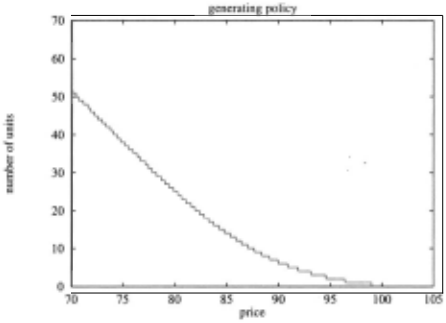
We have tested our approach on several sets of parameters. Figure 1 illustrates a typical policy. To find the zero points of expected added gain functions E(gk(p)), we used the basic Robbins-Monro algorithm for 10, 000 steps. We use the av­ erage of 100 runs. The thresholds were computed incremen­ tally starting from Pi. The interesting observation is that for larger values of k, thresholds become about equally spaced. In such a situation the policy can be more compactly rep­ resented using a linear function, directly mapping prices to recommended commodity holdings.

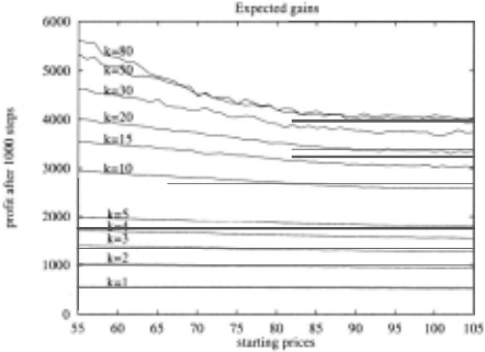
The effect of strategy refinement (adding more thresholds and potentially investing more units) on the quality of the so­ lution is illustrated in Figure 2. The results show average profit over 1000 runs for different policies and different start­ ing prices. We see that more complex policies with more thresholds tend to improve the profit performance initially. This effect becomes less significant for larger k's, and ex­ pected profits converge to the optimal value v· (p). Since the prices reach lower values very rarely, the probability of us­ ing thresholds for larger k 's is very small and corresponding more complex policies are only rarely utilized.

8 Conclusion

We have presented an efficient method for finding the near optimal policies for the commodity planning problem with trading and storage constraints. The problem has continuous state space and large action space and cannot be solved ef­ ficiently by standard dynamic programming solutions. Our solution relies on the analysis of the domain and takes advan­ tage of a problem structure and Monte Carlo approximation techniques. We showed that the optimal policy for the com­ modity trading problem with a mean-reverting price model and trading constraints can be represented compactly using a stack of decision (price) thresholds for investing in additional units of commodity. The thresholds correspond to zero points of expected added gain functions, which we also derived. As these functions do not have analytical solution, we ap­ ply Monte Carlo approximation techniques to find their zero points. The properties of the functions guarantee uniqueness of the solution and convergence of the approximation scheme.

Interesting questions and opened issues that remain to be addressed include the theoretical bound on the number of thresholds necessary to guarantee the near optimal strategy, and exploration of more compact parametric representations of the policy, mapping prices to the number of units to hold directly (these would eliminate the need to remember all threshold values). Finally, a number of interesting problems will arise if we relax some of the current assumptions of the model. Possible refinements may inClude price spreads, concurrent trading at multiple interconnected sites, or de­ mand/supply sensitive price models.

Acknowledgement

We wish to thank Oliver Frankel of Goldman Sachs for intro­ ducing us to this problem and for valuable technical discus­ sions.