
Multi-Value-Functions: Efficient Automatic Action Hierarchies for Multiple Goal MDPs
Proceedings of the Sixteenth International Joint Conference on Artificial Intelligence. Uncertainty and Probabilistic Reasoning. Pages 1316-1322.
© 1999 International Joint Conferences on Artificial Intelligence
Abstract
If you have planned to achieve one particular goal in a stochastic delayed rewards problem and then someone asks about a different goal what should you do? What if you need to be ready to quickly supply an answer for any possible goal? This paper shows that by using a new kind of automatically generated abstract action hierarchy that with N states, preparing for all of N possible goals can be much much cheaper than N times the work of preparing for one goal. In goal-based Markov Decision Problems, it is usual to generate a policy rr( x), mapping states to actions, and a value function J ( x), mapping states to an estimate of minimum expected cost-to-goal, starting at x. In this paper we will use the terminology that a multi-policy rr*(x, y) (for all state-pairs (x, y)) maps a state x to the first action it should take in order to reach y with expected minimum cost and a multi-valuefunction J* ( x, y) is a definition of this minimum cost. Building these objects quickly and with little memory is the main purpose of this paper, but a secondary result is a natural, automatic, way to create a set of parsimonious yet powerful abstract actions for MDPs. The paper concludes with a set of empirical results on increasingly large MDPs.
- [Bertsekas and Tsitsiklis, 1989] D. P. Bertsekas and J. N. Tsitsiklis. Parallel and Distributed Computation. Prentice Hall, 1989.
- [Chapman and Kaelbling, 1991] D. Chapman and L. P. Kaelbling. Learning from Delayed Reinforcement In a Complex Domain. In I JCAI-91, 1991.
- [Dayan and Hinton, 1993] P. Dayan and G. E. Hinton. Feudal Rein- forcement Learning. In S. J . Hanson, J . D Cowan, and C. L. Giles, editors, Advances in Neural Information Processing Systems 5.
- Morgan Kaufmann, 1993.
- [Dietterich, 1998] T. G. Dietterich. Hierarchical reinforcement learn- ing with the MAXQ value function decomposition. In Jude Shavlik, editor, International Conference on Machine Learning, 1998.
- L. Kaelbling. Hierarchicial Learning in Stochastic Domains: Preliminary Results. In Machine Learning: Proceedings of the Tenth International Workshop. Morgan Kaufmann, June 1993 .
- [Kearns et al., 1998] M. Kearns, Y. Mansour, and A. Ng. Sparse Sam- pling Methods for Planning and Learning in Large and Partially Observable Markov Decision •Processes. Draft Report, 1998.
- [Moore and Atkeson, 1993] A. W. Moore and C. G. Atkeson. Priori- tized Sweeping: Reinforcement Learning with Less Data and Less Real Time. Machine Learning, 13, 1993.
- [Moore, 1994] A. W. Moore. The Parti-game Algorithm for Vari- able Resolution Reinforcement Learning in Multidimensional State- spaces. In S. J. Hanson, J. D Cowan, and C. L. Giles, editors, Advances in Neural Information Processing Systems 6. Morgan Kaufmann, April 1994.
- [P arr and Russell, 1998] R. Parr and S. Russell. Reinforcement Learn- ing with Hierarchies of Machines. In Neural Information Processing Systems 10, 1997.
- Morgan Kaufmann, 1998.
- [Precup and Sutton, 1998] D. Precup and R. Sutton. Multi-Time Models for Temporally Abstract Planning. In Neural Information Processing Systems 10, 1997.
- Morgan Kaufmann, 1998.
- [Singh , 1991] S. P. Singh. Transfer of learning across compositions of sequential tasks. In L. Birnbaum and G. Collins, editors, Ma- chine Learning: Proceedings of the Eighth International Work- shop. Morgan Kaufmann, June 1991.
References were extracted automatically from the PDF and may contain errors.
Full text extracted automatically from the PDF; figures, tables and equations may differ. The PDF is the version of record.
1 Introduction
In goal-based Markov Decision Problems , it is usual to generate a policy and a value function for a single goal. In 1993, Kaelbling introduced the HDG (Hierarchical Distance to Goal) algorithm [Kaelbling, 1993], which considered the more general formalism of arbitrary goal states as well as start states. Given N states, HDG considered the question of how to generate and execute an approximation to the multi-policy without requiring O(N 2 ) memory for the data structures.
In this paper we introduce new data structures and algorithms that exploit this insight while automatically choosing where to place landmarks (points to aim for) , and choosing which states belong to which landmark, without requiring pre-defined distance metrics (such as the Euclidean heuristic of the original paper) or prede- Leslie Kaelbling Brown University lpk@cs.brown.edu fined partitions. Instead, the measure of closeness used is the true minimal expected cost measure. Generating these locations, partitions, and policies from scratch in volves some interesting "chicken and egg" problems, es pecially if we need to exploit the hierarchy whilst build ing it (necessary if we are to save not only memory but also computation). We will describe how this can be ad dressed with a new branch-and-bound procedure in com bination with prioritized sweeping [Moore and Atkesbn, 1993], an algorithm for improving value functions in the face of small alterations in an MDP structure.
Another motivation is to help answer the two ques tions, "Where should Abstract Actions come from?". Is it necessary to have some high-level prior understanding of the class of tasks at hand in order to decide which abstractions are beneficial? This may be of use to re cent algorithms that attempt to exploit abstract actions but require them to be predefined (such as [Precup and Sutton, 1998; Singh, 1991 ; Dayan and Hinton, 1993; Dietterich, 1998] and HDG itself).
2 The Airport Hierarchy
This algorithm takes, as input , an MDP which is spec ified by a set of N states , and for each state a set of actions, and for each state-action pair, a set of outcomes along with the outcome probabilities. The OUTCOMES() set of a state-action-pair (x , a) is the set of states { z} such that P ( next state = z ] this state = x, this action = a) > 0. We make the strong assump tion that the MDP is sparse: for all states the num ber of actions is < < N and for all state-action pairs, the number of outcomes is < < N. This assumption is very frequently true in navigation, dynamics and inven tory MDPs. Furthermore, recent work [Kearns et al., 1998] indicates that even non-sparse MDPs may usu ally be transformable to sparse MDPs with little loss in optimality. In addition to the state transition. proba bilities, the algorithm also inputs the non-negative one step cost function C(x, a) specifying the penalt.y we pay for applying a in state x. Note that conventiOnal dy namic programming theory tells us that the optimal policy and multi value function must obey J*(x , y) = minaQ*(x , y , a) and 1r*(x, y) = argminaQ*(x, y , a) where The new structure is called the Airport Hierarchy. It differs from HDG and is more similar to Feudal Learn ing [Dayan and Hinton, 1993] in that each state is a mem ber of many partitions: some large and abstract, others small and specific. It differs from Feudal Learning and other partitioning structures (such as G-leaming [Chap man and Kaelbling, 1991] and PartiGame [Moore, 1994]) in that junior partitions are not necessarily subsets of · their seniors, and many partitions are overlapping. We will begin by defining the properties that we do require from these partitions, before proceeding to execution and generation algorithms that exploit these properties. Proofs will be included in a later version of this paper.

2.1 Formalit ies
We define, for a given state y that we have decided to turn into an airport:
Any member of INS(y) will have, cached away in the air ports structure, knowledge of 7r*(x, y), the truly optimal first action to take in getting to y and J* ( x, y) , the true minimum expected cost of getting to y. Define
Where Level(y) = 0 means that y is a maximally senior airport: the larger the level, the lower the seniority. As part of the construction we will insist that
Thus, if y is a level i airport then there are at least N /2; states that know the optimal value and policy for reaching y. We also insist that
Thus, the set of n states that knows how to get to y are then states with minimal expected cost to get toy. Our final two requirements are
- If Level(y) 2 1 then INS(y) includes at least k senior air ports ( x is senior to z if and only if Level( x) < Level( z)).
- There are k airports at level 0, 2k at level 1, 4k at level 2, etc, with the number of airports doubling at each level until we run out of states.
Because the number of airports doubles at each level, the maximum level rises logarithmically with N. The total amount of memory needed to represent all knowl edge about all level i airports is thus, in the best case, O(N /2;) per airport times k2i level i airports, which is thus O(kN), and so the total amount of memory needed over all levels is O(kNlogN) in the best case.
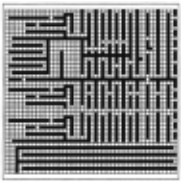
Example: Figures 1 and 2 depict aspects of the airport hierarchy for a simple grid-world.
2.2 Choosing Act ions
How is 7r*(x , y) approximated by the airport hierarchy? Call the approximation ir( x, y) . To choose the first ac tion to take if we hope eventually to reach y cheaply, we use the HDG insight. If x is far enough from y that it Figure 1: A simple maze con structed with k = 4 top-level airports. The light gray areas are cells in which transitions are completely random (to a random neighbor). In white cells, there is a 0.9 probability that we'll move in the direc tion (N, S, E or W) we request , and a Prand = 0.1 chance we'll move to a random neighbor. The disks denote the airports: the larger the disk, the more se nior the airport.
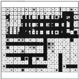
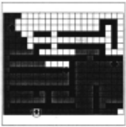
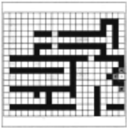
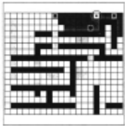
Figure 2: Each figure shows an airport y (circled) and INS(y) (dark grey). The air port levels are 1, 3 and 5 re spectively. The k = 3 senior airports that can reach the targets are also shown.
doesn't know how to get toy directly (i.e., if x tJ. INS(y)), we pick some intermediate target that we do know how to get to, and from which we will be able to make progress towards y. The only remaining question is how to choose a good target from the airport hierarchy.
To do this, we must define one extra object, called SINS(y), a special set of states that know how to get to y by travelling through increasingly less senior airports. Define
So that, for example, SINS 1 (y) consists of those states in INS(y) that happen to have a more senior airport level to Level(y) . Then write SINS(y) = Uk SIN:J<(y). Now we can define the target that x first aims for. We will deal in turn with three cases: states that immediately know how to get to y; states that are in SINS(y); and all other states.
- If x E INS(y) then define ir(x, y) = 7r*(x, y), and define J(x, y) = J*(x, y). These values can be read, in constant time, from the information cached in the airport hierarchy.
- If x rt INS(y), but x E SINS(y) then assume that x was entered into SINS(y) at level k + 1, so that x E SINSk+ 1 (y) but x rt SINSk(y). Then define
- Finally, if x rt INS(y) and x rt SINS(y) then define Common(x, SINS(y)) to be the set of states { z} such that x E INS( z) 1\ z E SINS(y). And then define
Common(x, SINS(y)) cannot be empty because SINS(y) must contain a Level 0 airport.
Intuitively, the process of creating SINS(y) can be seen as dynamically creating a goal-state-dependent set of landmarks (using HDG terminology) for getting to y. This set of landmarks is useful specifically for y be cause it has a higher density of landmarks closer to y (with closeness defined in terms of minimal expected cost). By construction (easy to prove) this set is small: O(k log2 N).
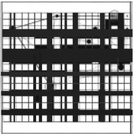
Figure 3 shows the set of airports considered during one such decision. Although the policies resulting from this scheme may be suboptimal, we can prove that they will always reach the goal in finite time, and empirically the regret (mean loss compared with truly optimal be havior) is very small.
2.3 Efficiently building the airport hierarchy
We say a state is unassigned if it is not an airport at any level in the hierarchy. The airport construction al gorithm begins with all states unassigned , and ends with no states unassigned. Whenever an airport y becomes assigned, Level(y) is chosen, the set INS(y) is chosen, and for all x E INS(y), J*(x, y) and 7r*(x, y) are com puted. All this information is cached permanently away in the airport hierarchy for future use during the remain ing airport construction and policy execution.
We will now discuss the AddAirport operation, which picks one state and assigns it.
2.4 Step One: Choose y
We defer discussion of this step until Section 2.7.
2.5 Step Two: Choose y's Level
This step is trivial. y is simply given the most senior air port level available , subject to the constraint that there are no more than k2L airports at level L. Thus, if so far, m airports have been assigned, y's level is log 2 (m/k).
2.6 Step Three: Construct INS(y)
To understand the job we must do here, we will be gin by considering two simplified scenarios: an ineffi cient method for non-deterministic MDPs and an ef ficient method for deterministic MDPs. Finally, we'll tackle the efficient non-deterministic case. ·
Constructing INS(y) inefficiently
We would simply take the following steps:
- Run an MDP solver such as value iteration, policy iteration, or modified policy iteration [Bertsekas and Tsitsiklis, 1989] to compute 7r*(x, y) and J*(x, y) for all states x in the MDP.
- Define the set BestsT (y) = {x such that J*(x, y) is among the T lowest values. }, with ties broken ar bitrarily to ensure r ·elements in the set. Define T* to be the minimum T such that T 2 N/2Level(y) and BestsT (y) contains at least k senior airports. Then simply select INS(y) = BestsT* (y) and store the J* ( x, y) and 7r* ( x, y) values in the airport hier archy only for those xs for which x E INS(y).
The objection to this approach is that it is too expen sive: after having computed the INS(y) set for every y in the MDP, we will have needed to perform N full dy namic programs, meaning O(N 2 kcrit) operations in total to build the hierarchy, where kcrit is the average num ber of value iterations needed for dynamic programming convergence.
Constructing INS(y) for deterministic systems
This too would be simple. We can perform uniform-cost breadth-first search back from y until the set of states added during the search become sufficiently large and contains the required number of senior airports. Now the work per airport would be small for junior airports with small INS(y) state sets, resulting in an algorithm that in the best case could be as cheap as O(N log N).
The efficient non-deterministic case
Again, we will work backwards from y, incremen tally adding states. The problem is that for a non deterministic system there is always a probability that the system being controlled will leave the set of states added so far. How, then, can we compute the optimal value function that takes into account the possibility of such exits?
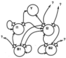
Let us briefly take a break from the larger question of computing INS(y), and instead focus on a simpler ques tion: given an incomplete portion of a goal-based MDP, how can we approximate J*(x, y) over the states in this incomplete portion (which we will callS)? Figure 4 gives an example of such a problem, with five states (including the goal state, Y) constituting S, and several outcomes that lead to states outside this set marked with ? sym bols . We will find an optimistic lower bound, } 0 Pt(x, y), and a pessimistic upper bound, Jpess(x, y) , on J*(x , y) so that
Constructing j 0 Pt(x, y)
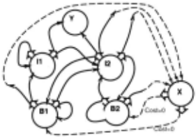
We will construct a new, small, MDP made up of the states in S, plus one new state X . This construction will be guaranteed not to overestimate J*(x, y) .
Before proceeding, we will partitionS into two subsets of states. Define
Internals { x E S such that V z E Preds( x) . z E S}
Borders
where z E Preds( x) means "z is an immediate predeces sor of x", so that z E Preds( x) - 3 a such that P( next state = x I this state = z and action =a) > 0.
Border states have some predecessor outside S, while internal states are ones in which all predecessors are in side S . In Figure 4, assume that Y, h, and h are all internal states, and B1 and B2 are border states.
For each of the ? symbols in Figure 4, what is the best thing that could happen? The first thought is that they might head straight to a state outside S, paying their one-step outcome cost, and then this state might be able to jump to the goal with zero cost. But this is not possible. If the goal is an internal state, then no state outside Scan jump directly to the goal, nor indeed to any other internal state. So the best thing that could happen is that they jump to some state outside S and then with zero cost jump to the most favorable of the border states. We model this by adding a new, fake , state called X to the system, which can with zero cost jump to any of the border states that it chooses . The ? symbols all jump to X . Figure 5 shows this construction for our example. Having added this extra state, we run an MDP solver to compute its value function , which we define to be Jopt (x , y) .
Constructing Jpess (x, y)
We must now ask "what 1s the worst thing that can
Figure 4: An example of a sub-MDP in the process of construction from five states S = {Y,J1,!2 , B1 , B2} · The thick polygonal arrows denote actions . The thin arrows denote the possible stochastic outcomes if the action is taken. Assume that all outcomes cost 1 unit , and for a given stateaction pair , all depicted outcomes are equiprobable.
happen at any of the ? symbols?". Unfortunately, it is arbitrarily bad. Even if there were an upper bound on a single transition cost in the MDP, hard-to-escape loops (caused by a probability-of-transition-to-self very close to 1) could create arbitrarily expensive expected costs to the goal.
The good news is that if Level(y) > 0, we may be able to take advantage of information cached in the partially constructed airport hierarchy. This requires that at least one state in S have already been added to the hierarchy as an airport , and that one or more other states in S know how to get to this airport.
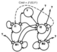
If there exists w E S and x E S such that w is an air port and x E INS( w) then we will add an extra action to x, with cost J*(x, w) (which we can look up in the hier archy) and with next state w with probability 1. Adding this action simply expresses the already established fact that we know we can get to w from x by some (not necessarily explicitly known) means, and the expected cost of doing so is J* ( x, w). Expressing this fact cannot { x E S such that 3z . z E Preds( x) I\ z rf. S} cause the system to underestimate the cost of travelling from x to y. Adding these new fake actions can have a dramatic effect on the worst case cost estimates. In Figure 4, the worst case value for all states other than Y is infinite. But suppose we add the extra knowledge that we already know that travelling from h to h costs, say, an expected 3 units (see Figure 6) . Then the op timal policy in the supplemented MDP will have costs Jpess(Jl, Y) = 5, Jpess(J2, Y) = 8, Jpess(Bl, Y) = 10 and Jpess(B2, Y) = 10.
Constructing INS(y)
We now return to the question of constructing INS(y) . The algorithm is:
- Let S = {y} , Borders= {y} , Internals= {} .
- Compute J opt(x, y) and Jpess(x , y) for all x E S using the modified versions of S described above.
Figure 6: The pessimistic interpretation of the subMDP of Figure 4, assuming that /2 E /NS(/1) .
- Define the set BestsT (y) = {x such that Jopt(x, y) is among the T lowest values } . Define T* to be the minimum T, if it exists, such that T ~ N/2Level(y) and BestsT (y) contains at least k senior airports. If such a T* exists, check the tightness on our lower and upper bounds on J*(x , y) for all states in BestsT* (y) . If
then halt, adding y into the airport hierarchy, along with its chosen level, and INS(y) = BestsT* (y), and remembering for future use all the J*(x, y) values for x E INS(y), approximating J*(x , y) by (Jopt(x, y) + Jpess(x, y))/2.
- If we did not halt, grow S. Pick the border state with minimum JOPt(x, y), add all its predecessors into S and Borders. Check which states have all their immediate predecessors in S and promote them into Internals. Goto 2.
Remarks:
Each time Jopt(x, y) and JPess(x, y) are recomputed, few of the states inS change their values significantly, except for newly added states and their neighbors. To take advantage of this, we use prioritized sweeping [Moore and Atkeson, 1993). This was used in the experiments reported in Section 3, and without it, the computational costs were empirically 5 to 100 times slower.
In order to access the immediate predecessors in the MDP, we must create a backwards model, which is an array which, for each state x, maps x to Preds(x). This can be built once, with a construction cost linear in the number of states.
Why should we expect that the upper and lower bounds on the value function will be tight? Not all domains will provide tightness: for example, expander graphs are likely to be problematic. But domains with a notion of locality are likely to achieve tight bounds on states close to the goal quite early on.
2. 7 Choosing airport locations
When the hierarchy is being built, level 0 airports are assigned first, then level 1, etc. The location of a new airport is always chosen to be the state furthest from any previous airport (in terms of expected cost). Because of the construction of the hierarchy, this can always be found efficiently. Notice that no prior assumptions (such as Euclidean distance) are needed for airport determina tion: it is fully automatic.
3 Results
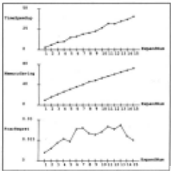
Table 1 presents results on various stochastic gridworlds and an inventory management problem. The gridworlds all obey the same rules as our initial example. Problems Expand1 through Expand15 are grid worlds of increasing size, produced by gluing together a short fat maze on top of itself. This allows us to see how costs increase as the maze size increases linearly. OneWay (middle of Figure 7) is a maze with one-way walls, and serves to demonstrate that it is not necessary for actions to be reversible for airports to be applicable. The table com pares the memory needed if a full1r(x, y) table were used to that needed by the airport hierarchy. It compares the time needed to build the airport hierarchy conventionally with the time needed using our algorithm. And it shows the mean regret (loss due to using our approximate pol icy, rr(x, y), instead of the optimal policy, 1r*(x, y)) . To give the regret some context it also shows the mean path cost. Figure 8 graphically depicts the tradeoff as the number of states is increased. Further empirical results, for which there is no room here, show that the algorithm work over a wide range of stochasticity, tha:t there is not strong sensitivity to the f threshold, and that clever placement of the airports is beneficial.
4 Conclusion
This paper has been about efficiently computing and caching a hierarchy that allows us to approximate J*(x, y) and 1r*(x, y) for all pair of states (x , y). When is this ability to access J* ( x, y) and 1r* ( x, y) useful? Cer tainly in domains in which we must perform multiple sequential tasks, and in which we need to very quickly switch from task to task. But we believe the greatest use will come in hierarchical control systems in which a higher level controller wishes to not merely call one of a set of atomic lower level controllers, but instead one of a set of lower level controllers that can be parameter ized with a subgoal. The full paper and presentation of this work includes an example of hierarchical control of hunters and prey which would not have been otherwise computationally feasible.
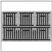
Figure 8: The relative perfor mance of using versus not using airports for different sizes of the Expand maze of Figure 7. Top graph: number of times by which the airports are faster than non airports in computing J*(x, y) and rr*(x, y). Middle graph: the num ber of times more memory that non-airports need. Bottom graph: the average regret of the airports policy, expressed as a fraction of path length.
| Name | Num States | Slow Memory (Wordsj | Airports Memory (Wordsj | Memory Saving Factor | Slow Time (sees) | Airports Time (sees) | Speed -up Factor | Mean J*(x, y) cost | Airports Mean Regret | Fraction Regret |
|---|---|---|---|---|---|---|---|---|---|---|
| Small | 246 | 0.061 | 0.011 | 5.4 | 18 | 7 | 2.6 | 30 | 0.28 | 0.009 |
| Medium | 1477 | 2.18 | 0.055 | 39.3 | 3064 | 2 16 | 14.2 | 39 | 0.46 | 0.012 |
| Big | 6480 | 41.990 | 0.700 | 60.0 | 69822 | 1429 | 48.9 | 104 | 0.51 | 0.005 |
| One Way | 1180 | 1.392 | 0.085 | 16.4 | 2301 | 219 | 10.5 | 99 | 2.84 | 0.029 |
| Inventory | 5313 | 28.228 | 2.507 | 11.3 | 55653 | 7518 | 7.4 | 62 | 6.90 | 0.111 |
| Expand! | 485 | 0.235 | 0.025 | 9.5 | 97 | 33 | 2.9 | 39 | 0.25 | 0.006 |
| Expand2 | 970 | 0.941 | 0.061 | 15.5 | 557 | 95 | 5.9 | 41 | 0.38 | 0.009 |
| Expand3 | 1455 | 2.117 | 0.102 | 20.8 | 1600 | 174 | 9.2 | 44 | 0.56 | 0.013 |
| Expa.nd4 | 1940 | 3.764 | 0.145 | 25.9 | 2570 | 258 | 10.0 | 49 | 0.76 | 0 .016 |
| ExpandS | 2425 | 5.881 | 0.191 | 30.8 | 4910 | 33 1 | 14 .8 | 52 | 0.74 | 0.014 |
| Expand6 | 2910 | 8.468 | 0.239 | 35.5 | 6838 | 424 | 16 . 1 | 55 | 1.27 | 0.023 |
| Expand7 | 3395 | 11. 526 | 0.289 | 39.9 | 10185 | 535 | 19.0 | 58 | 1.38 | 0.024 |
| Expand8 | 3880 | 15.054 | 0.330 | 45.6 | 12940 | 630 | 20.5 | 60 | 1.18 | 0.020 |
| Expand9 | 4365 | 19.053 | 0.395 | 48.3 | 16914 | 750 | 22.6 | 62 | 1.17 | 0.019 |
| Expand!O | 4850 | 23.523 | 0.446 | 52.8 | 22916 | 860 | 26.6 | 64 | 1.36 | 0.021 |
| Expand!! | 5335 | 28.462 | 0.502 | 56.7 | 30809 | 962 | 32.0 | 65 | 1.64 | 0.025 |
| Expandl2 | 5820 | 33.872 | 0.559 | 60.6 | 34774 | 1100 | 31.6 | 66 | 1.51 | 0.023 |
| Expandl3 | 6305 | 39.753 | 0.614 | 64.7 | 42243 | 1220 | 34.6 | 73 | 1.88 | 0.026 |
| Expandl4 | 6790 | 46.100 | 0.674 | 68.4 | 5 1643 | 1400 | 36.9 | 76 | 1.38 | 0.018 |
| Expandi5 | 7275 | 52.926 | 0.732 | 72.3 | 62746 | 1549 | 40.5 | 78 | 1.20 | 0.015 |
Multi-values are primitive in comparison with Parr's approach [Parr and Russell, 1998], which permits arbi trary reward functions instead of merely arbitrary goals. However, multi-value functions may be more computa tionally practical on large problems. Like other hierar chical RL algorithms, Airports uses abstract actions, and can be thought of as creating an entire plan, and then replanning on each time step. But Airports differs from other algorithms such as MAXQ [Dietterich, 1998) in the nature of those abstract actions, and this can be seen by looking at the plans produced. In MAXQ, the problem is solved by a sequence of Ievel-l actions. Each Ievel-l action is, in turn, a sequence of level-2 actions, and so on down to the level of primitive actions. The cost of a Ievel-l action is unknown until the lower levels have com puted. In Airports, the plan at a given time might be a single level-3 action ("go to this level-3 airport"), then a single level-7 action, then a single level-10 action. The sequence is constrained to always be in increasing numer ical order (decreasing levels of abstraction), with at most one action at each level, guaranteeing short plans. Each abstract action is composed directly of primitive actions, not lower-level abstract actions, and the complete hier archy of abstract actions-what they do and where they are applicable-is constructed automatically and parsi moniously. This restriction means that a good plan to get from state x to state y can be found by exhaustively searching all legal plans, and this is fast enough to be done in real time on every step. It might be interesting to combine airports with MAXQ or with Precup's and Sutton's abstract actions [Precup and Sutton, 1998], us ing the abstract actions generated by Airports as some of the "primitive" actions in the other algorithm.
@inproceedings{ijcai1999p187,
  title     = {Multi-Value-Functions: Efficient Automatic Action Hierarchies for Multiple Goal MDPs},
  author    = {Moore, Andrew W. and III, Leemon C. Baird and Kaelbling, Leslie Pack},
  booktitle = {Proceedings of the Sixteenth International Joint Conference on
               Artificial Intelligence, {IJCAI-99}},
  publisher = {International Joint Conferences on Artificial Intelligence},
  editor    = {Thomas Dean},
  pages     = {1316--1322},
  year      = {1999},
  note      = {Uncertainty and Probabilistic Reasoning},
  url       = {https://ijcai.org/proceedings/1999/187},
}
TY - CPAPER TI - Multi-Value-Functions: Efficient Automatic Action Hierarchies for Multiple Goal MDPs AU - Moore, Andrew W. AU - III, Leemon C. Baird AU - Kaelbling, Leslie Pack T2 - Proceedings of the Sixteenth International Joint Conference on Artificial Intelligence, IJCAI-99 PB - International Joint Conferences on Artificial Intelligence PY - 1999 SP - 1316 EP - 1322 UR - https://ijcai.org/proceedings/1999/187 ER -Copied
Machine-readable versions of this paper, for tools and AI agents:





