
On the Role of Context-Specific Independence in Probabilistic Inference
Proceedings of the Sixteenth International Joint Conference on Artificial Intelligence. Uncertainty and Probabilistic Reasoning. Pages 1288-1292.
© 1999 International Joint Conferences on Artificial Intelligence
Abstract
Context-specific independence (CSI) refers to conditional independencies that are true only in specific contexts. It has been found useful in various inference algorithms for Bayesian networks. This paper studies the role of CSI in general. We provide a characterization of the computational leverages offered by CSI without referring to particular inference algorithms. We identify the issues that need to be addressed in order to exploit the leverages and show how those issues can be addressed. We also provide empirical evidence that demonstrates the usefulness of CSI.
- [Boutilier et al., 1996] C. Boutilier, N. Friedman, M. Goldszmidt, and D. Koller, Context-specific inde- pendence in Bayesian networks, Proc. of 12th Con- ference on Uncertainty in AI, 115-123.
- [Cheuk and Boutilier, 1997] A. Y. W. Cheuk and C. Boutilier, Structured arc reversal and simulation of dynamic probabilistic networks, Proc. of 13th Con- ference on Uncertainty in AI, 72-79.
- [D'Ambrosio, 1994] B. D'Ambrosio, Local expression languages for probabilistic dependence, Int. J. of Approximate Reasoning, 11 (1), 1-16.
- [Dechter, 1996] R. Dechter, Bucket elimination: A uni- fying framework for probabilistic inference, Proc. of 12th Conference on Uncertainty in AI, 211-219.
- [Fung and Shachter, 1990] R. M. Fung and R. D. Shachter, Contingent Influence Diagrams, Ad- vanced Decision Systems, 1500 Plymouth St., Mountain View, CA 94043, USA.
- [Geiger and Heckerman, 1996] D. Geiger and D. Beck- erman, Knowledge representation and inference in similarity networks and Bayesian multimets, Artifi- cial Intelligence, 92, 45-7 4.
- [Howard and Matheson, 1984] R. A. Howard, and J . E. Matheson, Influence Diagrams, The principles and Applications of Decision Analysis, Vol. II, R. A. Howard and J. E. Matheson (eds.). Strategic De- cisions Group, Menlo Park, California, USA.
- [Jensen et al. , 1990] F. V. Jensen, K. G. Olesen, and K. Anderson, An algebra of Bayesian belief universes for knowledge-based systems, Networks, 20, 637 - 659.
- [Lauritzen and Spiegelhalter, 1988] S. L. Lauritzen and D. J. Spiegelhalter, Local computations with prob- abilities on graphical structures and their applica- tions to expert systems, Journal of Royal Statistical Society B, 50: 2, 157 -224.
- [Olmsted, 1983] S. M. Olmsted, Representing and solv- ing decision problems, Ph.D. Dissertation, Depart- ment of Engineering-Economic Systems, Stanford University.
- [Pearl, 1988] J . Pearl, Probabilistic Reasoning in Intel- ligence Systems: Networks of Plausible Inference, Morgan Kaufmann Publishers, Los Altos, CA.
- [Poole, 1997] D. Poole, Probabilistic partial evaluation: exploiting rule structure in probabilistic inference, Proc. of 15th Int. Joint Conference on AI, 1284- 1291. IJCAI
- [Quinlan, 1986] J. R. Quinlan , Induction of decision trees, Machine Learning, 1, pp. 81-106.
- [Santos Jr. and Shimony, 1996] E. Santos Jr. and S. E. Shimony, Exploiting case-based independence for approximating marginal probabilities, Int. J. of Ap- proximate Reasoning, 14, 25-54.
- [Shafer and Shenoy, 1990] G. Shafer and P. Shenoy, Probability propagation, Annals of Mathematics and AI, 2, 327-352.
- [Smith et al. , 1993] J. E. Smith, S. Holtzman, and J . E. Matheson, Structuring conditional relationships in influence diagrams, Operations Research, 41, No. 2, 280-297.
- [Zhang and Poole, 1996] N. L. Zhang and D. Poole, Ex- ploiting causal independence in Bayesian network inference, J. of AI Research, 5, 301-328.
- [Zhang, 1998] N. L. Zhang, Inference in Bayesian net- works: The role of context-specific indepen- dence, Technical Report, HKUST-CS98-09, De- partment of Computer Science, University of Sci- ence and Technology, Hong Kong. Available at http://www.cs.ust.hk/ lzhang/paper/csitr.html. Link
References were extracted automatically from the PDF and may contain errors.
Full text extracted automatically from the PDF; figures, tables and equations may differ. The PDF is the version of record.
1 Introduction
The theory of probabilistic inference begins with a joint probability over all variables of interest. The amount of numbers it takes to specify a joint probability is expo nential in the number of variables. For this reason, prob abilistic inference was thought to be infeasible until the introduction of Bayesian networks (BNs) [Pearl, 1988; Howard and Matheson, 1984]. Making use of condi tional independence, a BN factorizes a joint a probability into a list of conditional probabilities. The factorization renders inference computationally feasible in many ap plications because each of the conditional probabilities involves only a fraction of the variables.
In practice, there are often conditional independence relationships that are true only in specific contexts. The concept of context-specific independence ( CSI) was in troduced specifically for such relationships. CSI has its roots in the influence diagram literature [Olmsted, 1983; Fung and Shachter, 1990; Smith et al., 1993] and was first formalized by [Boutilier et al., 1996]. Researchers have shown that CSI can be exploited to speed up vari ous Bayesian network inference algorithms such as sym bolic probabilistic inference [D'Ambrosio, 1994], search [Santos Jr. and Shimony, 1996], cutset conditioning [Boutilier et al., 1996; Geiger and Beckerman, 1996], clique tree propagation (CTP) [Boutilier et al., 1996), arc reversal [Cheuk and Boutilier , 1997], and variable elimination (VE) [Poole, 1997].
David Poole
Department of Computer Science University of British Columbia Vancouver, BC V6T 1Z4, Canada poole~cs.ubc.ca
This paper results from efforts to identify the common principle underlying those works. We attempt to answer the following questions: Why in general CSI leads to faster inference? In other words, how do we characterize the computational leverages offered by CSI without re ferring to particular inference algorithms? What issues do we need to address in order to exploit the leverages? How do we address those issues? Finally, how much can we gain?
It is well known that the computational leverages af forded by conditional independence can be characterized in terms of factorization: conditional independence al lows one to factorizes a joint probability into a list of conditional probabilities. As it turns out, the computa tional leverages offered by CSI can also be characterized in terms of factorization. More specifically, CSI allows one to further decompose some of the conditional prob abilities, giving rise to a finer-grain factorization of the joint probability. This is precisely why CSI can speed up inference.
In order to take advantage of the finer-grain factoriza tion, the main technical issue that one needs to address is that some of the factors in the factorization are partial functions. Fortunately, this issue can easily be addressed using an operation called union-product. ·
In addition to providing a clear picture about the role of CSI in probabilistic inference, this paper also gives a general method for exploiting CSI. The method can be easily grounded with popular inference algo rithms such as CTP [Lauritzen and Spiegelhalter, 1988; Jensen et al., 1990; Shafer and Shenoy, 1990] and VE [Zhang and Poole, 1996; Dechter, 1996]. All one has to do is change one basic operation, namely replacing product of full functions with union-product of partial functions.
Experiments have been performed to empirically demonstrate the effectiveness of CSI. The results con firmed that CSI can significantly speed up inference.
2 Bayesian Networks and Probabilistic Inference
To start with, this section briefly reviews the concepts of Bayesian networks and factorization. We also explain why factorization is the key to efficient inference.
2.1 Bayesian Networks
A Bayesian network 1 (BN) is an annotated directed acyclic graph, where each node represents a random vari able and is associated with the conditional probability of the node given its parents. In addition to the explic itly represented conditional probabilities, a BN also im plicitly represents conditional independence assertions. Let x1 , x2 , ·. . , Xn be an enumeration of all the nodes in a BN such that each node appears before its chil dren and let 1l'xi be the set of parents of a node Xi . The following assertions are implicitly represented: Each variable Xi is conditionally independent of variables in {x1,x2, .. . ,xi-d\1l'xi given variables in 1l'zi·
The conditional independence assertions and the con ditional probabilities P(xil11'i) attached to the nodes to gether entail a joint probability over all variables. As a matter of fact, we have
where the first equality follows from chain rule and the second follows from the conditional independence asser tions.
2.2 Probabilistic Inference
Inference refers to the process of computing the posterior probability P(XIY=Yo) of a list X of query variables after obtaining some observations Y=Yo. Here Y is a list of observed variables and Yo is the corresponding list of observed values.
The posterior probability P(XIY =Yo) can be ob tained from the marginal probability P(X, Y), which in turn can be computed from the joint probability P(x1, x2, ... , Xn) by marginalizing out variables outside XUY one by one. Since a BN implicitly represents a joint probability, one can in theory perform arbitrary in ference. In practice, this is not viable because marginal izing out a variable from a joint probability requires an exponential number of additions.
1 Also known as probabilistic influence diagrams and belief networks.
The key to efficient inference lies in the concept of factorization. A factorization of a joint probability is a list of factors (functions) from which one can reconstruct the joint probability.
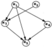
Because of (1), we say that a BN factorizes a joint probability P(x1, X2, ... , Xn) into conditional probabil ities p(x1111'x1 ), p(x211l'x 2 ), ·· · , and p(xnl11'xn) and that the conditional probabilities constitute a multiplicative factorization of the joint probability. The BN in Fig ure 1, for instance, gives us the following multiplicative factorization of P(x1, x2, ... , x5):
We will use this network as a running example through out the paper.
To see why factorization is of fundamental im portance to inference, consider a joint probabil ity P(x1, x2, ... , Xn) over n binary variables. To marginalize out a variable Xi means to compute L:xi P(x1, x2, ... , Xn). This computation is global since all variables are involved. It takes 2n- 1 numerical addi tions and hence is infeasible except when n is very small.
Now suppose we have a multiplicative factorization of the joint probability {It, /2, ... , f m} and only the first k factors involve· Xi· By distributivity, we have
Consequently, we can marginalize out Xi from the fac torization as follows:
- Remove from the factorization all functions that involve Xi ;
- Compute the product of the functions;
- Marginalize out Xi from the product; and
- Put the resulting function back to the factorization.
This is the principle underlying inference algorithms such as CTP and VE. Here one needs to compute L:xi rr;=l /j. This computation is local in the sense that it involves only some of the variables. It is usually much cheaper than the global computation mentioned above.
In our running example, marginalizing out x2 means to compute I:x 2 P(x1, x2, Xg, x4, x5) without factorization. This takes 16 additions. With factorization, on the other hand, one needs to compute I:., P(x2)P(xglx1,x2), which takes only 4 additions. 2
3 CSI and Decomposition of Conditional Probabilities
We next review the concept of CSI and shows how it leads to decomposition of conditional probabilities.
3.1 Context-Specific Independence
Let C be a set of variables. A context on C is an assign ment of one value to each variable in C. We denote a context by C="'f, where 'Y is a set of values of variables in C. Two contexts are incompatible if there exists a variable that is assigned different values in the contexts. They are compatible otherwise.
This following definition of CSI is due to [Boutilier et al., 1996]. Let X, Y, Z, and C be four disjoint sets of variables. X and Y are independent given Z in context C="f if
whenever P(Y, Z, C="()>O. When Z is empty, one sim ply says that X andY are independent in context C="(.
As an example, consider four variables: income, pro fession, weather, and qualification. A farmer's in come depends on weather and typically does not de pend on his qualification. On the other hand, a office clerk's income depends on his qualification and typically does not depend on weather. In other words, income is independent of qualification in the context "profes sion=farmer" and it is independent of weather in the context "profession=office-clerk".
3.2 Decomposition of Conditional Probabilities
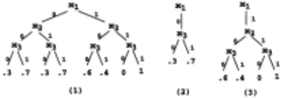
To illustrate how CSI leads to decomposition of con ditional probabilities, we use P(x3lxi,x2) as an exam ple. Consider P(x3lxi=O,x2) and P(x3lxi=1,x2) sepa rately. Assume X3 is independent of x2 in context Xi =0. Then P(x3lxi=O,x2)=P(x3lxi=O). Consequently, we can decompose P(x3lxi,x2), which requires 8 numbers to specify, into two smaller components P(x31xi=O) and P(x31xi =1, x2), which require only 6 numbers to specify.
To make the example more concrete, suppose P(x3lxi,x2) is given by the tree shown in Figure 2 (1). The tree states that P(x3=0ixi =0, x2=0), for in stance, is 0.3. Because X3 is independent of x2 in context Xi =0, the tree can be decomposed into the two smaller trees shown in Figure 2 (2) and (3), which represent P(x31xi =0) and P(x31xi =1, x2) respectively.
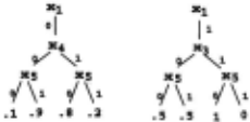
Next assume x5 is independent of X3 given X4 in con text Xi =0 and xs is independent of X4 given X3 in con text Xi=l. Then P(xslxi=O,x3,x4)=P(xslxi=O,x4) and P(xslxi =1, x3, x4)=P(xslxi =1, x3). Consequently, we can decompose P(xslxi,X3,x4), which requires 16 numbers to specify, into two smaller components P(xslxi=O,x4) and P(xslxi=1,x3), which take only 8 numbers to specify. For concreteness, assume the two smaller components are given by the trees in Figure 3.
After the decompositions, the decomposition given in (2) becomes
This decomposition is of finer-grain because the condi tional probabilities of X3 and x5 have be broken up into smaller pieces.
4 Making Inference with Refined Factorizations
This section shows how to make inference with factor izations such as the one given by (3). A technical issue that we need to address is that some of the factors are partial functions. For example, P(x31xi=O) is a partial function of Xi and X3 in the .sense that it is not defined for the case when Xi =1.
In general, a partial function of a set X of variables is a mapping from a proper subset of possible values of X to the real line. In other words, it is defined only for some but not all possible values of X. The set of possible values of X for which a partial function is defined is called the domain of the partial function. A full function of X is a mapping from the set of all possible values of X to the real line. In other words, it is defined for all possible values of X . In the rest of a paper, we will use the term "function" when we are not sure whether a function is a partial function or a full function.
4.1 Union-Product
To manipulate partial functions, we need the operation of union-product. Suppose X, Y, and Z are three dis joint sets of variables and suppose g(X, Y) and h(Y, ZJ are two functions. The union-product g'I!!Jh of g and h is the function of variables in XUYUZ given by
| (gi1lslh)(X, Y, Z)= | undefined | if both g(X, Y) & h(Y, Z) undefined if g(X, Y) defined, h(Y, Z) undefined |
| g(X, Y) | ||
| h(Y, Z) | if g(Y, Z) undefined, h(X, Y) defined | |
| g(X, Y)h(Y, Z) | if both g(X, Y) & h(Y, Z) defined |
The operation is illustrated in Figure 4. We sometimes write gi1lslh as g(X, Y)lilslh(Y, Z) to make explicit the ar guments off and g. When the domains of g and hare disjoint, we call g'r.tJh the union of g and h and write it as gUh.
2 The notation illsl is produced in LATEX using macro {\cup}\hspace{-0.6em}{·}.
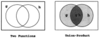
Here are some of the properties of the union-product operation. First, the union-product of two full functions is simply their product. Together with the concept of union, this explains the term "union-product" . Second, the union-product of a full function with another func tion, full or partial, is a full function. Third, the union product operation is associative and commutative. We can hence talk about the union-product of a list of func tions. The 1.mion-production of a list :F of functions will be denoted as bti:F.
4.2 Decompositions
The concept of union allows us to rigorously defined de composition. A list :F of functions with disjoint domains is decomposition of a function f iff= U :F. A decompo sition is proper if no two functions in the decomposition share the same set of arguments. A decomposition of a function f is nontrivial if at least one function in the de composition has fewer arguments than f itself. A func tion is decomposable if it has a nontrivial decomposition.
The function shown in Figure 2 (1) is decomposable. It can be nontrivially decomposed into the the two partial functions shown in Figure 2 (2) and (3) .
4.3 Union-Product Factorizations
With union-product, we can now make explicit the sense in which the list of functions given in (3) is a factorization of the joint probability P(x1, x2, X3, x4, xs) .
A list :F of functions is a union-product factorization, or simply a UP-factorization, of a function f if f=bti:F. Note that functions in a decomposition must have dis joint domains whereas domains of functions in a UP factorization might intersect. A decomposition is a UP factorization but not vice versa.
For any variable x, let :Fx be the set of functions in :F that contain x as an argument. A UP-factorization :F is normal if bti:Fx is a full function whenever :Fx=f-0.
The list of function given in (3) is a factorization of the joint probability P(xt,x2,x3,x4,xs) because
- P(x1, x2, X3, x4, xs),
where the first equality is true because the union product operation is associative, the second equality fol lows from the assumptions made in Section 3, and the third equality follows from the first property of union product. The factorization is also normal. For example, :Fx3 ={P(x31Xt =0), P(x3lx1 =1, x2), P(xslxt =1, x3)}. Since P(x3lx1 =O)Ic!siP(x3lx1 =1, xz)=P(x31Xt , xz) is a full function, so must be bti:Fx 3 by the second property of union-product.
In general, let :F be the set that consists of, for each variable in a BN, the conditional probability of the vari able or, when the conditional probability is decomposed, its components. Then :F is a normal UP-factorization of the joint probability of all variables. It is of finer-grain than the multiplicative factorization given by the BN if at least one conditional probability is decomposed.
4.4 Inference with UP-Factorizations
The following theorem, which we state without proof, lays the foundation for making inference with normal UP-factorizations.
Theorem 1 Suppose :F is a normal UP-factorization of a full function f and x is an argument of f. Then Q=(:F \ :Fx)U{l:x bti:Fx} is a normal UP-factorization of Lxf·
According to the theorem, a variable x can be marginalized out from a normal UP-factorization as fol lows:
- Remove from the factorization all functions that involve x;
- Compute the union-product of the functions;
- Marginalize out x from the union-product; and
- Put the resulting func;tion back to the factorization.
Comparing this procedure with the one outlined in Sec tion 2, we see that existing inference algorithms such as CTP and VE can be adapted to work with normal UP factoiizations by simply replacing product of full func tions with union-product of partial or full functions .
The above descriptions are rather abstract. For ex ample, implementations of union-product and marginal ization are not given. Those and other details can be found in a longer version of the paper [Zhang, 1998]. In that paper, the method is also compared to previous methods.
5 CSI and Inference Efficiency
Using the running example, this section illustrates why inference with finer-grain UP-factorizations is more efficient than with the corresponding multiplicative factor izations.
Consider marginalizing out x3 . Without CSI, we need to compute
With CSI, we need to compute
The second computation is cheaper than the first one for a number of reasons. The conditional probability P(x3lx1, x2 ) is decomposed into two components that takes fewer numbers to specify. The conditional proba bility P(x5lx1,x3,x4) is also decomposed into two com ponents that take fewer numbers to specify. Moreover, only one of those two components is involved in the sec ond computation. As a consequence, the second com putation has fewer variables (x4 not involved) and fewer numbers to deal with.
In general, marginalizing out a variables from a finer grain UP-factorization involves fewer variables and fewer numbers than with the corresponding multiplicative fac torization. It is therefore cheaper.
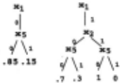
There is another reason why finer-grain UP factorizations leads to faster inference. The result of expression (5) is a full function of x1 and x5 . The full function happens to be decomposable and can be de composed into the two partial functions shown in Figure 5. In such a case, we can compute the decomposition directly. This is less expensive than computing the full function itself because the decomposition requires fewer numbers to specify.
When we compute decompositions of functions instead of functions themselves, we are preserving structures. Preserving structures not only benefits the current step of inference but also simplifies future steps. It is there fore an important issue. In [Zhang, 1998), this issue is addressed in detail.
6 Empirical Results
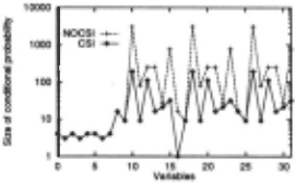
Experiments have been conducted to demonstrate the computational benefits of CSI. A BN named Water was used in the experiments 3 . Water is a model for the bio logical processes of a water purification plant. It consists of 32 variables. Strictly speaking, conditional probabil ities of the variables are not decomposable. To make them decomposable, some of the probability values were modified. The induced errors are upper bounded by 0.05. Using a decision-tree-like algorithm [Quinlan, 1986], we were be able to decompose some of the modified condi tional probabilities and thereby reduce their representa tion complexities drastically 4 . See Figure 6.
3 0btained from a Bayesian network repository at Berkeley.
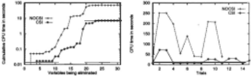
The experiments were based on the VE algorithm and were performed on a SUN ULTRA 1 machine. The task was to eliminate all variables according to a predeter mined elimination ordering. In the first experiment, an ordering by Kjrerullf was used 5 . The the amounts of times in CPU seconds that VE took, with and without CSI, to eliminate the first n variables for n running from 0 to 31 are shown in left chart of Figure 7. We see that VE ran much faster with CSI. In particular, the en tire elimination process took about 7 seconds with CSI. Without CSI, however, it took about 70 seconds.
In the second experiment, we generated 14 new elim ination orderings by randomly permuting pairs of vari ables in Kjrerullf's ordering. A trial was conducted with each ordering. The performances of VE, with and with out CSI, across all the trials are summarized in the right chart of Figure 7. We see that VE was significantly more efficient with CSI than without CSI. The speedup was more than one magnitude on average. Moreover, there are four trials where VE was not able to complete without CSI due to large memory requirements. With CSI, on the other hand, VE completed each of those four trials in less than 30 seconds.
4 Modifications of probability values actually take place during the decomposition process. We choose to describe them as two separate steps here for presentation clarity.
5 The ordering was also obtained from the Berkeley repository.
7 Conclusions
This paper studies the role of CSI in Bayesian network inference. It differs from earlier work in that we do not attempt to demonstrate the usefulness of CSI in partic ular inference algorithms. Rather, we provide a general characterization of the computational leverages offered by CSI. This characterization fits well with the char acterization of the computational leverages afforded by conditional independence. They both are in terms of factorization. While conditional independence provides one with a factorization of a joint probability, CSI allows one to refine the factorization.
We clearly identify the issues that one needs to ad dress in order to takes advantage of the computational leverages offered by CSI. There are two issues: partial functions and preservation of structures. The first issue in addressed in detail and the second issue is addressed in [Zhang, 1998]. We also give a general method for ex ploiting CSI. The method can be easily grounded with popular inference algorithms such as CTP and VE. All one has to do is to replace product of full functions with union-product of partial and full functions. Finally, we provide empirical evidence that demonstrates the useful ness of CSI.
Acknowledgements
The authors thank the anonymous reviewers for use. ful comments and suggestions. Research is supported by Hong Kong Research Grants Council Grant HKUST6125/98E and Natural Sciences and Engineer ing Research Council of Canada Research Grant OG P0044121.
@inproceedings{ijcai1999p183,
  title     = {On the Role of Context-Specific Independence in Probabilistic Inference},
  author    = {Zhang, Nevin Lianwen and Poole, David},
  booktitle = {Proceedings of the Sixteenth International Joint Conference on
               Artificial Intelligence, {IJCAI-99}},
  publisher = {International Joint Conferences on Artificial Intelligence},
  editor    = {Thomas Dean},
  pages     = {1288--1292},
  year      = {1999},
  note      = {Uncertainty and Probabilistic Reasoning},
  url       = {https://ijcai.org/proceedings/1999/183},
}
TY - CPAPER TI - On the Role of Context-Specific Independence in Probabilistic Inference AU - Zhang, Nevin Lianwen AU - Poole, David T2 - Proceedings of the Sixteenth International Joint Conference on Artificial Intelligence, IJCAI-99 PB - International Joint Conferences on Artificial Intelligence PY - 1999 SP - 1288 EP - 1292 UR - https://ijcai.org/proceedings/1999/183 ER -Copied
Machine-readable versions of this paper, for tools and AI agents:





