
Decision Tree Grafting From the All Tests But One Partition
Proceedings of the Sixteenth International Joint Conference on Artificial Intelligence. Machine Learning. Pages 702-706.
© 1999 International Joint Conferences on Artificial Intelligence
Abstract
Decision tree grafting adds nodes to an existing decision tree with the objective of reducing prediction error. A new grafting algorithm is presented that considers one set of training data only for each leaf of the initial decision tree, the set of cases that fail at most one test on the path to the leaf. This new technique is demonstrated to retain the error reduction power of the original grafting algorithm while dramatically reducing compute time and the complexity of the inferred tree. Bias/variance analyses reveal that the original grafting technique operated primarily by variance reduction while the new technique reduces both bias and variance.
- Bauer & Kohavi, in press] E. Bauer & R. Kohavi. An empirical comparison of voting classification algo- rithms: Bagging, boosting, and variants. Machine Learning, in press.
- [Blake, Keogh, & Merz , 1998] C. Blake, E. Keogh, & C. J. Merz. UCI repository of machine learning databases. [Machine-readable data repository]. Uni- versity of California, Department of Information and Computer Science, Irvine, CA., 1998.
- [Breiman, 1996] L. Breiman. Bagging predictors. Ma- chine Learning, 24:123-140, 1996.
- [Freund & Schapire, 1996] Y. Freund & R. E. Schapire. Experiments with a new boosting algorithm. In Pro- ceedings of the Thirteenth International Conference on Machine Learning, pages 148-156, Bari, Italy, 1996.
- [Morgan Kaufmann. Geman, Bienenstock, & Doursat , 1992] S. Geman, E. Bienenstock, & R. Doursat. Neural networks and the bias/variance dilemma. Neural Computation, 4:1-48, 1992.
- [Kohavi & Wolpert, 1996] R. Kohavi & D. Wolpert. Bias plus variance decomposition for zero-one loss functions. In Proceedings of the 13th International Conference on Machine Learning, pages 275-283, Bari, 1996.
- Morgan Kaufmann. [Quinlan, 1991]
- J . R. Quinlan. Improved estimates for the accuracy of small disjuncts. Machine Learning, 6: 93-98, 1991.
- [Quinlan, 1996] J . R. Quinlan. Bagging, boosting, and C4.5. In AAAI-96, 1996.
- [Quinlan, 1998] J. R. Quinlan. Miniboosting decision trees. Submitted for publication, August 1998.
- [Quinlan & Cameron-Jones, 1995] J. R. Quinlan & R. M. Cameron-Jones. Oversearching and layered search in empirical learning. In IJCAI'95, pages 1019- 1024, Montreal, 1995. IJCAI
- Morgan Kaufmann.
- [Webb, 1996] G. I. Webb. Further experimental evi- dence against the utility of Occam's razor. Journal of Artificial Intelligence Research, 4:397-417, 1996.
- [Webb, 1997] G. I. Webb. Decision tree grafting. In IJCAI-97: Fifteenth International Joint Conference on Artificial Intelligence, pages 846-851, Nagoya, Japan, August 1997.
- Morgan Kaufmann.
References were extracted automatically from the PDF and may contain errors.
Full text extracted automatically from the PDF; figures, tables and equations may differ. The PDF is the version of record.
1 Introduction
Decision committee techniques, notably AdaBoost [Fre und & Schapire, 1996] and bagging [Breiman, 1996] have demonstrated spectacular success at reducing decision tree error across a wide variety of learning tasks [Quin lan, 1996; Bauer & Kohavi, in press]. These techniques apply a base learning algorithm multiple times to form a committee of classifiers. All committee members vote to classify an unseen case. The success of these approaches has demonstrated that there is room to improve upon the average case prediction performance of standard de cision tree learning algorithms. However, decision com mittees deliver this improvement at a cost. Whereas a single decision tree provides a model that is straight forward to interpret, comprehension of a decision com mittee requires juxtaposition of all constituent models . This is infeasible in non-trivial cases. While it is possi ble to construct a single decision tree that expresses the model inherent in a decision committee, for even small committees there is an exponential increase in the size of the derived single tree model relative to the unmodified model of the base learning algorithm [Quinlan, 1998]. For any but the most simple of domains, this will reduce ease of comprehension critically.
Decision tree grafting has been presented as a tech nique that obtains some of the benefit of a decision com mittee while creating only a single tree [Webb, 1997].
Grafting is applied as a postprocess to an inferred de cision tree. It identifies regions of the instance space that are not occupied by training examples, or occupied only by misclassified training examples, and considers alternative classifications for those regions. Support for those classifications is obtained by considering alterna tive branches that could have been selected at ancestor nodes to the leaf containing the region in question. If those alternative branches indicate stronger support for an alternative classification than that assigned to the region by the current tree, a new branch is grafted to the tree that imposes the new classification on the re gion. While the increase in tree complexity of this tech nique is much lower than that of forming a single tree from a committee, the average increase in accuracy is also lower. Also, initial techniques were limited in ap plication to continuous valued attributes. This paper presents extensions to decision tree grafting that extend grafting to discrete valued attributes; dramatically re duce induction time; reduce the complexity of inferred trees; and increase average prediction accuracy. It also provides a bias/variance analysis of grafting's error re duction, demonstrating that the original algorithm re duced error primarily through variance reduction while the new algorithm reduces both bias and variance.
2 Previous Grafting Algorithms
The first decision tree grafting algorithm, C4.5X, was developed to investigate the utility of Occam's razor [Webb, 1996]. It was not initially conceived as a prac tical learning technique. The success of the technique at reducing prediction error led to further development aimed at creating a practical learning algorithm. This led to C4.5+, a postprocessor for C4.5 Release 8, that demonstrated frequent, if modest, reductions in predic tion error from that of the unmodified C4.5 over a wide cross-selection of learning tasks [Webb, 1997].
Appendix A presents C4.5++, the C4.5+ grafting algo rithm extended in a straight-forward manner to handle discrete valued attributes. This algorithm investigates in turn each leaf of an existing tree. For each leaf, l, and attribute a, it climbs the tree investigating at ancestor nodes for l alternative cuts on a that would project across the region of the instance space encompassed by l . It assesses for each such alternative cut the evidence that it would have presented about the class of objects that fall within its projection across l, if selected instead of the cut actually imposed at the ancestor. If that evidence provides stronger support for an alternative classification to the support for the original classification at the leaf, the new cut is saved for possible imposition. When all such cuts have been identified at ancestors of l, they are ordered and imposed on l from best supported to least. Support for a classification from a leaf or cut is obtained by applying the Laplace accuracy estimate
where pos(X, c) is the number of members of the set of training examples X that belong to class c.
While C4.5++ is reasonably consistent at reducing the error of classical decision tree induction, the technique has a number of deficiencies. One of these is its com putational complexity. The complexity of the algorithm is O(l · d · a· t), where l is the number of leaves in the initial tree, d is the maximum depth of the tree, a is the number of attributes, and t is the number of training cases. Where these values are large, application of the algorithm can become infeasible. Much of the efficiency of decision tree learning is derived from the manner in which it partitions the data so that, for the majority of processing (at the leaves) , only very small subsets of the training data need be considered. In contrast, C4.5+ and C4.5++ require consideration of all training data that reaches each ancestor of each leaf, once for each attribute for each leaf. Hence, the entire training set (the data at the root) must be processed once for each combination of attribute and leaf.
A further concern is that grafting considers very large numbers of possible grafts, which must substantially in crease risk of overfitting the data. That is, there is a substantial risk of finding grafts that appear good by chance. This can be viewed as a form of oversearch ef fect [Quinlan & Cameron-Jones, 1995].
Finally, one of the justifications for grafting is that it allows non-local information (examples from outside the leaf) to be considered when deciding how to classify regions within the leaf that are occupied by few or no training examples. However, the manner in which exter nal examples may be used is determined by where in the tree they are located relative to a leaf, rather than where in the instance space they fall. Hence, it is likely that an example, e, that is very close to a region, r, being in vestigated will have little influence on the classification that is selected if e happens to be divided from r by a cut close to the root of the decision tree. A training case separated by a single cut closer to the leaf l that contains r will have greater influence on the class selected for r, as it will be considered at every ancestor of l as the al gorithm climbs the tree. A training case x that fails all tests leading to l will have as much influence as a case y that fails only the test at the root of the tree, even though y may directly adjoin r and x fall at the opposite end of the instance space. Both will be considered once only, when the algorithm considers cuts that could have been imposed at the root of the tree.
3 Grafting from the all-tests-but-one partition
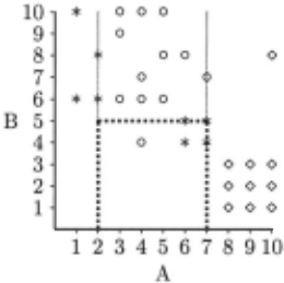
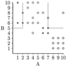
Grafting requires a means of estimating the accuracy of a potential new leaf that contains few or no training cases. Quinlan (1991] uses the context to estimate the accuracy of a leaf with few training cases. This context is called herein the all-tests-but-one-partition (ATBOP). The ATBOP of a leaf l is the region of the instance space that is separated from the region covered by l by no more than one decision surface. It will be reached by any case that fails no more than one test on a path from the root of the tree to l. This region is illustrated in Figures 1 and 2. The first figure, replicated from Webb (1997], provides a representation of a simple two attribute instance space projected as a two-dimensional geometric space. Objects of three classes are represented by *, o, and o, where each of these symbols represents a different class. The dashed lines represent the decision boundaries created by the decision tree (presented in Table 1) generated by C4.5 Release 8 for this training data. Points on a vertical line are included in the region to its left and points on a horizontal line are included in the region below. The region projected in Figure 2 is the ATBOP for the leaf highlighted in Figure 1. As these figures illustrate, the
A > 7 : 0 (10.0) A <= 7 : I A <= 2 * (4.0) I A > 2 : I I B <= 5 * (5. 0/1. 0) I I B > 5 : 0 (11.0)ATBOP for a leaf l is the region formed by removing all and only the decision surfaces that enclose l.
This paper explores the use in decision tree grafting of estimation within the ATBOP instead of estimation at ancestor nodes.
Using the ATBOP to evaluate the evidence support ing alternative classifications of a region within a leaf has a number of advantages over using ancestor nodes. Computational requirements are greatly reduced. Only one set of data is considered at any leaf l (the cases in the ATBOP of l), rather than one set for each ancestor of l . Further, that data set cannot be larger and will usually be considerably smaller than the largest data set used by the original technique-all training data, consid ered at the root. A further advantage is that the order in which decision boundaries have been imposed by the learning algorithm will not affect the outcome, a cut at the root is treated identically to the deepest cut within a tree. This appears better motivated than the original technique. Finally, the number of alternative cuts that are evaluated is considerably reduced, decreasing the op portunity for chance overfitting of the training data.
The resulting algorithm is identical to C4.5++, as pre sented in Appendix A, except that Steps 2a and 3a are each replaced by
n: n is the all-test-but-one-partition of l
4 Experimental evaluation
To evaluate the utility of the new grafting technique, four algorithms-C4.5, C4.5+, C4.5++, and C4.5A were compared on 34 data sets from the UCI reposi tory [Blake, Keogh, & Merz , 1998]. These data sets include all of those employed in previous grafting re search [Webb, 1996; 1997] augmented by a wide cross selection of discrete valued data sets. Note that the data sets employed in the earlier studies slightly disadvantage grafting as they include the discordant and sick data sets that were specifically added because they were variants of hypo, the only data set on which C4.5 outperformed C4.5X in the first experiment conducted. These are the only data sets selected due to specific predictions about the performance of grafting, and those predictions were that grafting would not perform well.
All four algorithms were implemented as a single mod ified version of C4.5 release 8 that incorporates all vari ations as options. In each case grafting was applied to pruned decision trees, as previous evaluation has sug gested that this provides the best average-case performance [Webb, 1997]. All experiments were run on a SUN Ultra 2 Model 2295 with dual 295 MHz CPUs.
The performance of an algorithm on a data set was evaluated by ten rounds of three-fold cross validation. In each round, the data were divided into three sub sets. For each subset s in turn, a decision tree was learned from the remaining two subsets and evaluated by application to s. This procedure was used to sup port estimation of bias and variance. Variance measures the degree to which the predictions of different learned classifiers vary as a result of differences in the training data. Variance impacts on error, as if different predic tions (of a single test item) are made as a result of dif ferent training data, not all can be correct, and so errors must result. Bias measures the error due to the central tendency of the learning algorithm. Kohavi & Wolpert's [1996] bias/variance decomposition was selected for this study as it is both applicable to multiple class domains and close to the original bias/variance decomposition for numeric regression [Geman, Bienenstock, & Doursat , 1992]. Some analyses also consider intrinsic noise, the minimum possible error for a domain, but this research followed Kohavi & Wolpert by aggregating this quantity into bias. The use of ten rounds of three-fold cross val idation replicated Kohavi & Wolpert's bias/variance es timation technique except that cross-validation was sub stituted for random sampling, ensuring that all available items were used the same number of times for training (20 times). Each item was also used the same number of times for testing (10). This uniformity in the number of times an item was utilized in each role can be expected to produce greater consistency across different runs of the procedure. Under Kohavi & Wolpert's original pro cedure, a given training example x might be used any number between zero and 30 times for training and any of zero, 10, 20, or 30 times for testing. This variability can be expected to increase the (statistical) variance of the measures obtained for accuracy, bias, and (learning) variance.
Table 2 presents the mean error (number of misclas sifications divided by total classifications) of the thirty trees learned and evaluated in this manner for each com bination of learning algorithm and domain. The last row of this table presents the mean error across all data sets. As can be seen, all grafting techniques narrowly outper form plain C4.5 on this latter measure. However, this measure should be treated as indicative only, as it is not clear to what extent error rates across different data sets are commensurable.
Table 3 presents specific comparisons of each pair of learning algorithms. Each algorithm is represented by three rows in the table. The first row, labeled i:, presents the geometric mean error ratio of each other algorithm against the nominated algorithm. This is the geomet ric mean 1 of cjr, where cis the error for the algorithm All data sets
1 The geometric mean of a set of values x1 to Xn is vT1~=l,. X;. This provides a better aggregate evaluation of a set ot ratio outcomes than arithmetic mean as if the geo-
| Data Set | C4.5 | C4.5+ | C4.5++ | C4.5A |
|---|---|---|---|---|
| anneal | 0.097 | 0.086 | 0.086 | 0.087 |
| audio | 0.255 | 0.255 | 0.257 | 0.254 |
| autos | 0.253 | 0.248 | 0.246 | 0.245 |
| balance-scale | 0.222 | 0.213 | 0.213 | 0.221 |
| breast cancer Slov. | 0.294 | 0.294 | 0.290 | 0.294 |
| breast cancer Wise. | 0.056 | 0.051 | 0.051 | 0.054 |
| Cleveland | 0.254 | 0.241 | 0.239 | 0.248 |
| credit (Aust .) | 0.147 | 0.146 | 0.148 | 0.145 |
| credit (German) | 0.282 | 0.283 | 0.279 | 0.280 |
| discordant | 0.012 | 0.013 | 0.013 | 0.012 |
| echocardiogram | 0.286 | 0.285 | 0.285 | 0.286 |
| glass | 0.352 | 0.344 | 0.344 | 0.345 |
| heart | 0.238 | 0.226 | 0.229 | 0.234 |
| hepatitis | 0.206 | 0.192 | 0.194 | 0.200 |
| horse-colic | 0.165 | 0.165 | 0.165 | 0.165 |
| house-votes-84 | 0.050 | 0.050 | 0.050 | 0.049 |
| Hungarian | 0.213 | 0.209 | 0.208 | 0.211 |
| hypo | 0.005 | 0.006 | 0.006 | 0.005 |
| iris | 0.063 | 0.064 | 0.064 | 0.061 |
| kr-vs-kp | 0.008 | 0.008 | 0.007 | 0.008 |
| labor-neg | 0.209 | 0.209 | 0.209 | 0.209 |
| lenses | 0.204 | 0.204 | 0.204 | 0.204 |
| lymphography | 0.228 | 0.228 | 0.220 | 0.224 |
| new-thyroid | 0.082 | 0.088 | 0.088 | 0.076 |
| Pima diabetes | 0.264 | 0.260 | 0.260 | 0.263 |
| primary tumor | 0.618 | 0.618 | 0.617 | 0.618 |
| promoters | 0.239 | 0.239 | 0.226 | 0.235 |
| segment · | 0.041 | 0.049 | 0.049 | 0.039 |
| sick | 0.013 | 0.015 | 0.015 | 0.014 |
| sonar | 0.280 | 0.259 | 0.269 | |
| soybean | 0.102 | 0.259 | 0.100 | 0.102 |
| large splice junction | 0.068 | 0.102 | 0.081 | 0.067 |
| tic-tac-toe | 0.163 | 0.068 0.163 | 0.163 | 0.160 |
| waveform | 0.276 | 0.264 | 0.264 | 0.267 |
0.184 0.181 0.180
0.181
to which a column relates, and r is the error for the algorithm to which the row relates. A value below 1.0 indicates an advantage to the algorithm for the column. A value above 1.0 indicates an advantage to the algorithm for the row. The row labeled s indicates the win/ draw /loss record. The three numbers for each entry indicate the number of data sets for which c < r , c = r, and c > r, respectively. The row labeled p indicates the two-tailed 2 binomial probability of obtaining the relevant win/loss outcome by equiprobable chance.
C4.5+ achieves lower error than C4.5 for twice as many data sets as the reverse, but the geometric mean error ratio very slightly favors C4.5. It is notable, however, that this latter result can be attributed mainly to the single hypo data set, for which the error differs by only
metric mean indicates an advantage in the error for algorithm a over that for algorithm b then it will also indicate a disadvantage for b over a. Arithmetic mean does not have this desirable antisymmetry with respect to ratios of outcomes.
2 Two tailed tests are used for consistency throughout because predictions were not made for the outcomes of some pairwise comparisons.
| Algorithm | C4.5 r p r | C4.5+ 1.001 14/13/7 0.189 | C4.5++ o.999 20/5/9 0.061 0.998 | C4.5A o.984 23/10/1 < 0.001 0.983 |
| C4.5 | s | |||
| C4.5+ | s p r | 10/19/5 0.302 | 15/7/12 0.701 0.985 | |
| C4.5++ | s p | 12/3/19 0.281 |
0.001, but C4.5's error is so low that this results in a very high error ratio. If hypo were excluded, the geometric mean error ratio would be 0.93 in favor of C4.5+. While the win/ draw /loss record is not statistically significant, many of the data sets do not contain continuous value attributes, denying C4.5+ a chance to alter the perfor mance of C4.5.
Both C4.5++ and C4.5A outperform C4.5 on both ge ometric mean error ratio and win/loss/draw record, the latter advantage being statistically significant at the 0.05 level on a two-tailed sign test for C4.5A but not C4.5++ 3 .
C4.5A outperforms C4.5++ on geometric mean error ratio, but C4.5++ achieves lower error than C4.5A for more data sets than the reverse. This latter advantage is not statistically significant at the 0.05 level, however. These results do not suggest that either C4.5A or C4.5++ holds a strong advantage in general error performance over the other.
Table 4 presents the relative bias performance of the algorithms. Only aggregate results are presented due to space constraints. This table follows the format of Table 3 with an additional row labeled Mean that cor responds to the final row of Table 2. While the means across all data sets vary only slightly, the other compar ative statistics suggest that C4.5 enjoys a slight general advantage over C4.5+ and C4.5++ (although not statisti cally significant at the 0.05 level) and that C4.5A enjoys a small but consistent and significant (at the 0.05 level) advantage over C4.5 and a small advantage over C4.5+ and C4.5++ that approaches significance at the 0.05 level.
Table 5 presents the algorithms' relative variance per formance. All the grafting algorithms enjoy a small but consistent and significant advantage over C4.5 in this re spect. Both C4.5+ and C4.5++ enjoy an advantage over C4.5A, this being statistically significant at the 0.05level for C4.5++. There is a straight forward explanation .for this outcome. The original grafting techniques allow cuts that could have been imposed high in the tree to be su perimposed further down the tree. If small variations in the training data lead C4.5 to different selections of attribute for nodes high in a tree, variance is likely to be enhanced. The superimposition of those alternative cuts at lower levels in the tree by grafting will counteract this upwards influence on variance. C4.5A, by not consider ing the data at ancestor nodes has less opportunity to superimpose such cuts, but may do so as a consequence of supporting evidence for the cut in the ATBOP.
3 As it was predicted that C4.5++ would outperform C4.5, it could be argued that a one-tailed sign test should be em ployed, in which case the outcome of 0.031 would be signifi cant at the 0.05 level.
| Algorithm Mean | C4.5 0.119 i: | C4.5+ 0.119 1.021 7/15/12 | C4.5++ 0.120 1.026 11/6/17 0.345 | C4.5A 0.118 0.995 15/15/4 0.019 |
| C4.5 | s p | 0.359 | ||
| C4.5+ | i: s p i: | 1.005 6/19/9 0.607 | 0.975 16/11/7 0.093 0.969 | |
| C4.s++ | s p | 19/7/8 0.052 |
| Algorithm Mean | C4.5 0.065 i: | C4.5+ 0.061 0.944 | C4.5++ 0.061 0.939 | C4.5A 0.063 0.969 |
| C4.5 | s p | 18/15/1 < 0.001 | 23/7/4 < 0.001 | 22/11/1 < 0.001 |
| C4.5+ | i: s p | 0.994 8/23/3 0.227 | 1.026 10/8/16 0.327 | |
| C4.s++ | i: s p | 1.031 6/8/20 0.009 |
Table 6 analyses the comparative complexity (mea sured by number of nodes) of the trees produced by each algorithm. All the grafting algorithms consistently in crease complexity (as they must). C4.5A consistently produces less complex trees than the previous grafting algorithms. The mean complexity of the trees produced by C4.5A is approximately twice that of C4.5 whereas the ratio for C4.5++ is more than 7 to 1.
A major advantage of C4.5A is a reduction in compu tational complexity in comparison to the original graft ing algorithms. The average compute times for the four systems are C4.5: 0.095; C4.5+: 4.239, C4.5++: 4.422; and C4.5A: 0.165 CPU seconds. For the grafting al gorithms these times include both induction of the ini tial tree and postprocessing to produce the final tree, and hence are consistently greater than those for C4.5. Times exclude reading the training or test data from disk but include application of the classifier to the test data and minor overheads associated with measuring bias and variance. For no data set did C4.5A more than triple the compute time of C4.5. The greatest increase in compute time due to the other grafting algorithms was for the segment data set for which both required 112 times the compute time of the original C4.5.
| Algorithm Mean | C4.5 38.0 | C4.5+ 106.7 | C4.5++ 281.9 3.378 | C4.5A 64.1 |
| C4.5 | i: s p | 1.965 0/11/23 < 0.001 | 0/1/33 < 0.001 | 1.451 0/4/30 < 0.001 |
| C4.5+ | i: s p | 1.719 0/13/21 < 0.001 | 0.739 23/1/10 0.035 0.430 | |
| C4.s++ | i: s p | 33/1/0 < 0.001 |
5 Summary and Conclusions
Grafting from the ATBOP has demonstrated a number of advantages over previous grafting algorithms. With out signficantly affecting error performance, grafting from the ATBOP dramatically reduces compute times and the size of inferred trees. Grafting has not previ ously been evaluated in terms of bias and variance. The current studies revealed that the previous grafting tech niques operated primarily be variance reduction. Graft ing from the ATBOP is slightly less effective at variance reduction than the previous techniques, but introduces a compensating bias reduction effect. The bias/variance operational profile of the original grafting techniques is similar to that of bagging in that it reduces variance only [Bauer & Kohavi, in press]. In contrast, ATBOP grafting has a bias/variance reduction profile similar to boosting in that it reduces both bias and variance [Bauer & Ko havi, in press]. While the error reduction effect of graft ing is of much smaller magnitude than that of bagging or boosting, ATBOP grafting produces a single decision tree which will usually be much more straight forward to interpret than the committees of decision trees pro duced by boosting and bagging. In consequence, grafting deserves serious consideration for machine learning ap plications where it is desirable to minimize error while producing a single comprehensible classifier.
A C4.5++ Algorithm
Let cases(n) denote the set of all training cases that can reach node n, unless there are no such cases in which case cases(n) shall denote the set of all training cases that can reach the parent of n.
Let value(a, x) denote the value of attribute a for training case x .
Let pos(X, c) denote the number of objects of class c in the set of training cases X.
Let class(x) denote the class of object x .
Let Laplace(X, c) = poj~~~+l where X is a set of training cases, lXI is the number of training cases and cis a class.
Let upperlim(n, a) denote the minimum value of a cut con continuous attribute a for an ancestor node x of n with re spect to which n lies below the a :5 c branch of x . If there is no such cut, upperlim(n, a) = oo. This determines an upper bound on the values for a that may reach n.
Let lowerlim(n, a) denote the maximum value of a cut con continuous attribute a for an ancestor node x of n with re spect to which n lies below the a> c branch of x. If there is no such cut, lowerlim(n, a) = -oo. This determines a lower bound on the values for a that may reach n.
Let prob(x, n,p) be the probability of obtaining x or more positive objects in a random selection of n objects if the prob ability of selecting a positive object is p.
To post-process leaf l dominated by class c
- Initialize to {} a set of tuples t containing potential tests.
- For each continuous attribute a
- (a) Find values of
n: n is an ancestor of l
v : 3x : x E cases(n) & v = value(a,x) & v :::; min(value(a,y): y E cases(l) & class(y) = c) & v > lowerlim(l, a)
k: k is a class
that maximize C' = Laplace({x: x E cases(n) & value(a,x):::; v & value(a,x) > lowerlim(l,a)},k).
- (b) Add to t the tuple (n, a, v, k, C', :5)
- (c) Find values of
v: 3x: x E cases(n) & v = value(a,x) & v > max(value(a,y): y E cases(l) & class(y) =c) & v :5 upperlim(l,a)
- n: n is an ancestor of l k: k is a class
that maximize C' = Laplace( {x : x E cases(n) & value(a,x) > v & value(a,x) :5 upperlim(l ,a)},k) .
- (d) Add tot the tuple (n,a,v,k,C',>)
- For each discrete attribute a for which there is no test at an ancestor of l
- (a) Find values of
- n : n is an ancestor of l v: v is a value for a k: k is a class
that maximize C' = Laplace( {x : x E cases(n) & value(a,x) = v}, k) .
- (b) Add tot the tuple (n,a,v,k,C',=)
- Remove from t all tuples (n, a, v, k, C, x) such that C :::; Laplace(cases(l), c) or prob(x, n, Laplace(cases(l), c)) :5 0.05.
- Remove from t all tuples (n, a, v, c, C, x) such that there is no tuple (n', a', v', k', C', x') such that k' # c & C' < C.
- For each (n, a, v, k , C, x) in t ordered on C from highest to lowest value
If xis:::; then
- (a) replace l with a node t with the test a :5 v .
- (b) set the :5 branch for t to lead to a leaf for class k.
- (c) set the > branch for t to lead to l .
- else if x is > then
- (a) replace l with a node t with the test a :5 v.
- (b) set the > branch for t to lead to a leaf for class k.
- (c) set the :::; branch for t to lead to l.
else (x must be=)
- (a) replace l with a node t with the test a= v.
- (b) set the = branch fort to lead to a leaf for class k.
- (c) set the# branch fort (implemented as a C4.5- subset branch) to lead to l .
@inproceedings{ijcai1999p100,
  title     = {Decision Tree Grafting From the All Tests But One Partition},
  author    = {Webb, Geoffrey I.},
  booktitle = {Proceedings of the Sixteenth International Joint Conference on
               Artificial Intelligence, {IJCAI-99}},
  publisher = {International Joint Conferences on Artificial Intelligence},
  editor    = {Thomas Dean},
  pages     = {702--706},
  year      = {1999},
  note      = {Machine Learning},
  url       = {https://ijcai.org/proceedings/1999/100},
}
TY - CPAPER TI - Decision Tree Grafting From the All Tests But One Partition AU - Webb, Geoffrey I. T2 - Proceedings of the Sixteenth International Joint Conference on Artificial Intelligence, IJCAI-99 PB - International Joint Conferences on Artificial Intelligence PY - 1999 SP - 702 EP - 706 UR - https://ijcai.org/proceedings/1999/100 ER -Copied
Machine-readable versions of this paper, for tools and AI agents:





