
Constructive Induction: A Version Space-based Approach
Proceedings of the Sixteenth International Joint Conference on Artificial Intelligence. Machine Learning. Pages 708-712.
© 1999 International Joint Conferences on Artificial Intelligence
Abstract
By automatically reformulating the problem domain, constructive induction ideally overcomes the defects of the initial description. The reformulation presented here uses the Version Space primitives D(E, F), defined for any pair of examples E and F, as the set of hypotheses covering E and discriminating F. From these primitives we derive a polynomial number of M-of-N concepts. Experimentally, many of these concepts turn out to be significant and consistent. A simple learning strategy thus consists of exhaustively exploring these concepts, and retaining those with sufficient quality. Tunable complexity is achieved in the MONKEI algorithm, by considering a usersupplied number of primitives D(Ei, Fi), where E; and F; are stochastically sampled in the training set. MONKEI demonstrates good performances on some benchmark problems, and obtains outstanding results on the Predictive Toxicology Evaluation challenge.
- Anglano et al., 1998)
- C. Anglano, A. Giordana, G. LoBello, and L. Saitta. An experimental evaluation of coevolutive concept learning. In J . Shavlik, ed., Proc. of the 1Sh ICML., pages 19-27.
- Morgan Kaufmann, 1998.
- Breiman et al., 1984) L. Breiman, J.H. Friedman, R .A. 01- shen, and C.J . Stone. Classification and Regression by tree. Wadsworth, Belmont California, 1984.
- C. Blake and Merz, 1998) E. Keogh C. Blake and C.J . Merz. UCI R epository of machine learning databases. http:/ fwww.ics . uci.edu/ "'mlearn/MLRepository.html, 1998. Link
- Craven and Shavlik, 1993) M.W . Craven and J .W. Shavlik. Learning to represent codoris: A challenge problem for constructive induction. In Proc. of IJCAI-g3, pages 1319- 1324.
- Morgan Kaufmann, 1993.
- Dietterich , 1998)
- T .G. Dietterich. Approximate statistical tests for comparing supervised classification learning algo- rithms. Neural Computation, to appear, 1998.
- Freund and Shapire, 1996)
- Y. Freund and R .E. Shapire. Ex- periments with a new boosting algorithm. In Proc. of the l:fh ICML ., pages 148-156.
- Morgan Kaufmann, 1996.
- Gama, 1998)
- J. Gama. Local cascade generalization. In J . Shavlik, ed., Proc. of th e 1Sh ICML., pages 206-214.
- Morgan Kaufmann, 1998.
- Haussler, 1988)
- D. Haussler. Quantifying inductive bias : AI learning algorithms and Valiant's learning framework. Artificial Intelligence, 36:177-221 , 1988.
- Holte, 1993)
- R.C. Holte. Very simple classification rules perform well on most commonly used datasets. Machine Learning, 11:63-90, 1993.
- Khardon and Roth, 1997) R. Khardon and D . Roth. Learn- ing to reason . Jal of the ACM, 44(5) :697-725, 1997.
- Kramer et al., 1998) S. Kramer, B. Pfahringer, and C.- Helma. Stochastic propositionalization of non-determinate background knowledge. In D. Page, ed., Proc. of Inductive Logic Programming'98, pages 29-61, 1998.
- Michalski, 1983)
- R.S . Michalski. A theory and methodology of inductive learning. In R.S Michalski, J .G. Carbonell, and T .M. Mitchell, eds, Machine Learning: an artificial in- telligence approach, volume 1, pages 83-134.
- Morgan Kauf- mann, 1983.
- Mitchell, 1982)
- T .M. Mitchell. Generalization as search. Ar- tificial Intelligence, 18:203-226, 1982.
- Muggleton, 1995)
- S. Muggleton. Inverse entailment and PROGOL. N ew Gen. Comput., 13:245-286 , 1995.
- Murphy and Pazzani, 1991) P.M. Murphy and M.J . Paz- zani . Id2-of-3: Constructive induction of M-of-N concepts for discriminators in decision trees. In L.A . Birnbaum and G.C. Collins, eds, Proc. of the ffh IWML, pages 183-187.
- Morgan Kaufmann, 1991.
- Perez and Rendell, 1995) E. Perez and L.A. Rendell. Using multidimensional projection to find relations. In Proc. of the lffh ICML ., pages 447-455.
- Morgan Kaufmann, 1995.
- Pitman, 1993)
- J. Pitman. Probability. Springer Verlag, 1993.
- Quinlan , 1990)
- J .R . Quinlan. Learning logical definition from relations. Machin e Learning, 5:239-266, 1990.
- Quinlan, 1993)
- J.R. Quinlan. C4.5: Programs for Machine Learning. Morgan Kaufmann, 1993.
- Schi:ilkopf et al. , 1998) B. Schi:ilkopf, C. Burgess, and A. Smola. Advances in Kernel Methods. MIT Press, 1998.
- Sebag and Rouveirol , 1997)
- M. Sebag and C. Rouveirol. Tractable induction and classification in FOL via Stochas- tic Matching. In Proc. of IJCAI-97, pages 888-892.
- Mor- gan Kaufmann, 1997.
- Sebag, 1996)
- M. Sebag. Delaying the choice of bias: A dis- junctive version space approach. In L. Saitta, ed., Proc. of the l:fh ICML., pages 444-452.
- Morgan Kaufmann, 1996.
- Srinivasan, 1997) A. Srinivasan. The predictive toxicology evaluation challenge. In Proc. of IJCAI-97, pages 4-8. IJCAI
- Morgan Kaufmann , 1997.
- Srinivasan, 1999) A. Srinivasan. PTE-Challenge, 1999. http://www .comlab.ox.ac. uk/ oucl/ groups/ machlearn/PTE. Link
- Weiss and Hirsh, 1998) G.M. Weiss and H. Hirsh. The prob- lem with noise and small disjuncts. In J . Shavlik, ed., Proc. of the Jsth ICML ., pages 574-578.
- Morgan Kauf- mann, 1998.
- Wnek and Michalski, 1994) J. Wnek and R.S . Michalski. Discovering representation space transformations for learn- ing concept descriptions combining DNF and M-of-N rules. In T. Fawcett, ed., Workshop on Constructive Induction, ICML-94 , 1994.
- Wolpert and Macready, 1995) D.H. Wolpert and W.G. Macready. No free lunch theorems for search. Technical report, Santa Fe Institute, 1995.
- Zilberstein, 1996)
- S. Zilberstein. Resource-bounded reason- ing in intelligent systems. Computing Surveys, 28( 4), 1996.
References were extracted automatically from the PDF and may contain errors.
Full text extracted automatically from the PDF; figures, tables and equations may differ. The PDF is the version of record.
1 Introduction
The goal of Machine Learning (ML) is to find a set of hypotheses accurately describing the target concept at hand, and to do so with an acceptable complexity: This is made possible only if the learner, the description of the problem domain and the distribution of the training examples fit well together.
When learning small disjuncts [Holte, 1993] for in stance, the difficulty might come from the distribution of the examples, and the existence of rare cases [Weiss and Hirsh, 1998]. It might also be due to the lack of rel evant primitives in the problem description [Perez and Rendell, 1995]- and indeed new primitives might allow to generalize/cluster rare cases in such a way that they are not "rare" any more. Last, the existence of rare cases might be caused by the learning strategy, e.g. based on set-covering [Michalski, 1983].
Constructive induction traditionally focuses on re fining (rewriting) the problem description [Michalski,
1983]. The quality of a reformulation is measured by the improvement of some base learner accuracy. Indeed, expert-driven reformulations of the problem domain can significantly improve the learning performances [Craven and Shavlik, 1993].
Constructive induction is the process of automatically finding a good quality reformulation. A first possibil ity is to derive the candidate reformulations from rules learned in a previous learning step. Wnek and Michalski [1994]look for new attributes allowing one to compact the previous rules. Gama [1998] uses the prediction of previously learned classifiers as new attributes. Another possibility is to syntactically define the space of candi date reformulations. For instance, MRP explores a set of relational patterns, defined as boolean functions of the initial attributes of the problem domain [Perez and Ren dell, 1995]. In first order logic, SP searches a set of boolean functions, used to rewrite first-order examples in propositional form [Kramer et al., 1998].
These approaches strongly depend on the quality of the knowledge provided to the system (through rules, classifiers or syntactic definitions of the candidate refor mulations), which must be relevant and make the search tractable.
To alleviate this limitation, we present a three-step approach interleaving induction and constructive induc tion: first, some initial hypotheses are constructed from the examples; second, these hypotheses incur a simple reformulation; last, some simple concepts of the refor mulated problem are considered, and those satisfying the validation criteria (minimal number of covered examples, maximal number of allowed exceptions) are retained.
This way, the learning workload might be balanced be tween constructive induction (reformulation) and induc tion, making it possible to relax their respective require ments: the quality of the initial hypotheses might be low, as these will be reformulated; the complexity of the reformulation might be low, as it is based on hypothe ses instead of examples; the last induction step might be rough, as simple worthy concepts are emerged by refor mulation. Only attribute-value languages will be consid ered in the paper.
This approach is rooted in the Version Space (VS) framework, which canonically characterizes the hypotheses solutions of a learning problem [Mitchell, 1982]. In order to give a polynomial characterization of the VS, we have introduced the primitives D(E, F) of the VS, de fined as the set of hypotheses covering any given example E and discriminating any example F [Sebag, 1996] (Sec tion 2). Indeed, D(E, F) can be viewed as the logical analog of the set of hyper-planes separating E from F.
The point here is that D(E, F) naturally gives rise to an integer attribute noted he,F (Section 3). Simple concepts built on this attribute (e.g. [he,F = M]) cor respond to M -of-N concept& of the initial domain lan guage. Reformulating the problem domain according to these attributes thus gives access to a polynomial-sized subset of the exponential set of all M -of-N concepts. Ex perimentally, it turns out that many of these concepts are worthy, i.e. they cover a significant number of ex amples, and are (almost) consistent. It is then sufficient to evaluate all candidate concepts, and retain those with acceptable significance and consistency.
However, if all primitives D(E, F) were considered, the complexity of the approach would be cubic in the number of examples, making it unrealistic to handle medium-to-large datasets. This paper thus presents an algorithm called MONKEI (for M-of-N-based Konstruc tivE Induction), using stochastic heuristics to achieve re source bounded induction, along the lines of bounded re source reasoning [Zilberstein, 1996]: the number of con sidered primitives D(E;, F;) is set by the user, and ex amples E; and F; are randomly selected in the training set (Section 4).
Our approach is situated with respect to related work (Section 5), and MONKEI is experimentally validated (Section 6). The advantage of this approach is success fully demonstrated on some problems in the Irvine repos itory [C. Blake and Merz, 1998], and a real-world prob lem proposed as an IJCAI challenge [Srinivasan, 1997], known as Predictive Toxicology Evaluation II.
The main limitation of MONKEI is that it provides a DNF theory, less intelligible than standard CNF theo ries. How to address this limitation, and other perspec tives of research, are discussed in the last section.
2 The primitives of Version Space
We assume the reader's familiarity with the Version Space framework [Mitchell, 1982] and its limitations due to an exponential complexity [Haussler, 1988]. As a gen eral remark, the complexity of a concept is commanded by its representation: a concept in DNF form (expressed as a conjunction of disjunctions) corresponds to an expo nential concept in CNF form (expressed as a disjunction of conjunctions). One way of having an affordable level of complexity (for both inductive and deductive reason ing) might thus be the use of a DNF formalism instead of a CNF one [Khardon and Roth, 1997].
Along these lines, the Disjunctive Version Space pro poses a polynomial DNF characterization of the Version Space [Sebag, 1996]. This characterization is built from elementary hypotheses D(E, F), called Version Space primitives: D(E, F) is defined as the set of all hypothe ses covering E and rejecting F , where E and Fare two distinct training examples.
We restrict ourselves to attribute-value logic, where hypotheses are conjunctions of selectors [att E Interval] and [att = value] respectively built on numerical ·and nominal attributes att. In this language, the upper bound of D(E, F) is the disjunction (the set) of all maximally general selectors covering E and rejecting F , termed maximally discriminant selectors [Michalski, 1983]. For instance in Table 1, [Att3 < 7.28] is the max imally discriminant selector built on attribute Att3.
By abuse of notations, D(E, F) is equated to its upper bound, hence characterized with linear complexity in the number of attributes.
| Att1 | Att2 | Att3 | Att4 | Att5 | Att6 |
|---|---|---|---|---|---|
| E Yes | 0 | 3.45 | 25 | red | ? |
| F No | 0 | 7.28 | 18 | ? | blue |
Let H be a conjunction of selectors, and assume that H belongs to the version space; by definition H is com plete (covers all positive training examples) and consis tent (rejects all negative examples). It follows that H be longs to (is subsumed by at least one selector in) D(E, F) for E ranging over the set £+ of positive examples and F ranging over the set &- of negative examples:
Inversely, let Q denote the above conjunction of D(E, F). One can show with no difficulty that all max imally general (conjunctive) hypotheses in Q are com plete and consistent. The version space and Q thus have same upper bound, and Q is expressed in DNF form with quadratic complexity in the number of examples and lin ear complexity in the number of attributes.
Other limitations of Version Spaces due to noisy and sparse data, or disjunctive target concepts, are dealt with by using parameterized combinations of the D(E, F) [Se bag, 1996].
3 Learning M -of-N Concepts
This section describes new attributes derived from the Version Space primitives and uses them to reformulate the problem domain. An overview of the MONKEI al gorithm is then presented.
3.1 Separating concepts
Let £ denote the attribute-value logic description of the problem domain (hypothesis and example language), de fined by numerical and/or nominal attributes.
Let E and F be two training examples, and let D(E, F) be constructed as in Section 2, as the set (dis junction) of N maximally discriminant selectors Sel;.
From D(E, F) we derive a mapping hE,F from the prob lem domain £ onto the set of integers: for each example or hypothesis U, hE,F(U) simply counts the number of selectors Seli that are satisfied by (covers) U. hE,F (or h when no ambiguity can arise) maps £ onto [0, N]: it defines a new computable attribute of the domain.
| Att1 | Att2 | Att3 | Att4 | Att5 | AttB | hE,F | |
|---|---|---|---|---|---|---|---|
| E | Yes | 0 | 3.45 | 25 | red | ? | 3 |
| F | No | 0 | 7.28 | 18 | ? | blue | 0 |
| u | ? | 1 | 5.28 | 20 | ? | blue | 2 |
Consider the selectors built on attribute h, (e.g. [h = M]), termed concepts. By definition, concept [h = M] corresponds to the M-of-N concept of selectors Seli: an example U satisfies [h = M] (equivalently, h(U) = M) iff U satisfies exactly M selectors among the S eli.
By construction, concepts [h = 0], ... , [h = N] are disjoint and define a partition of the examples.
Attribute hE,F can conveniently be viewed as a new discrete "dimension" of the problem domain. This di mension separates E from F, as these examples belong to opposite regions along this dimension: E belongs to [hE,F = N] since E satisfies all Seli; and F belongs to [hE,F = 0] since F satisfies none of the Seli.
3.2 Properties
Concepts [h = M] constitute a very flexible hypothe sis language, ranging from conjunctive hypotheses (e.g. [h = N] is conjunctive), to XOR patterns (e.g. [h = 1] corresponds to the XOR of selectors Seli)·
Note that concepts [h = M] can cover examples that are syntactically very different, inducing thereby unusual clusters of examples; this might hopefully decrease the number of "rare" cases.
Further, the distribution of the examples along dimen sion h (i.e. the number of examples covered by [h = M], for M E [0, N]) shows an interesting characteristic. If the initial attributes were independent, with probability Pi for any example to satisfy a given selector Seli, the Central Limit Theorem shows that the distribution of examples along h tends toward a Gaussian law of mean l:Pi when N goes to infinity (the approximation being considered accurate for N > 30 [Pitman, 1993]). The concepts [h = M] in the tails of the distribution (M close to 0 or N) would then cover few or no examples.
As could have been expected, experiments show that the initial attributes are not independent: concepts in the tails of the distribution happen to cover a significant number of examples. Further, these concepts happen to be consistent, i.e. all or most covered examples belong to the same class. As concepts [hE,F = M] are, sufficiently often, significant and consistent, a simple learning strat egy is to exhaustively explore these concepts, and retain all those that are sufficiently good. Further instances U are then classified by a majority vote of the concepts covering U.
The number of such new attributes hE,F is quadratic in the number P of examples; evaluating each hE,F on the training set is linear in the number of attributes and in the number of examples. Hence, the complexity of the exhaustive strategy is cubic in the number of ex amples, making it unrealistic to handle medium-to-large datasets.
3.3 Overview of MONKEI
Tunable complexity is achieved in MONKEI by consid ering a user-supplied number d of primitives D(Ei, Fi), where Ei and Fi are iteratively selected in the training set. The pairs of examples (Ei, Fi), called seed exam ples, are sampled by a stochastic boosting mechanism, based on the notion of margin. Within a majority vote based classifier, the margin of a training example E is the number of votes for the right class, minus the num ber of votes for the other class (or the second best class, in case of a multi-class discrimination problem) [Freund and Shapire, 1996]: E is misclassified iff its margin is negative.
In MONKEI, one of the seed examples, say Ei, is se lected with uniform probability among low-margin ex amples (i.e., whose margin according to the current the ory T h of the system is less than 1 through the follow ing). The other seed example is selected with uniform probability among the training examples that do not be long to the same class as the first seed example.
After a seed pair (Ei, Fi) has been selected, the corre sponding attribute h is computed for all training exam ples, and its domain [0, N] is discretized in K intervals h, ... ,IK (concepts [h = M] and [h = M +1] are merged if they cover examples in the same class). Each concept [h E Jk] is evaluated; it is added to the current theory if it covers more than a prescribed number A of examples and admits less than a prescribed rate c of exceptions 1 ; h is then termed dimension of the domain.
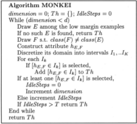
| Algorithm MONKEI |
| dimension= 0; Th = {}; IdleSteps = 0 |
| While (dimension< d) |
| Draw E among the low margin examples |
| If no such E is found, return Th |
| Draw F s.t. class(F) f. class(E) |
| Construct attribute hE F |
| Discretize its domain i~to intervals ! 1 , .. IK |
| For each h If [hE,F E h] is selected, Add [hE,F E Jk] to Th |
| If at leas.t one [hE,F E h] is selected, IdleSteps = 0 |
| Increment dimension |
| Else increment IdleSteps |
| If IdleSteps > T return Th End while return Th |
It might happen that many pairs of seed examples (Ei, Fi) are considered and no concept is retained; these steps are named "idle steps". The number of idle steps increases as learning proceeds, as there are less and less low-margin examples, and less chances to cover previ ously misclassified examples.
1 We further require the concept to cover at least one so far misclassified or unclassified example.
MONKEI repeatedly selects pairs of examples until the desired number of dimension d is reached, or the number of consecutive idle steps reaches a threshold T (set to 100 through the following).
Complexity. The worst case learning complexity is O(d x T x N x P), where d stands for the user-supplied number of dimensions, T is tl~e maximal number of con secutive idle steps allowed, P is the number of training examples, and N is the number of initial attributes.
At most d x N concepts are learned. As classifying U re quires to compute hE,,F, (U) only once (with complexity O(N)), the classification complexity finally is O(d x N).
4 Discussion
MONKEI explores a set of concepts that express some relations of the initial attributes, e.g. by counting the number of particular features that are simultaneously satisfied. Compared to the relational patterns used in MRP [Perez and Rendell, 1995], the difference is that the concepts explored here are automatically and poly nomially derived from the examples, and no preliminary discretization of numerical domains is required.
The constructed M-of-N concepts are simply evaluated; as opposed to MRP [Perez and Rendell, 1995] or ID2-of-3 [Murphy and Pazzani, 1991], MONKEI does not consider their combination (conjunction).
MONKEI must also be compared to Support Vector Machines (SVMs) [Scholkopf et al., 1998], which refor mulate the problem domain using kernel functions de rived from the examples. In the new description space, SVMs look for a separating surface optimizing the min imal margin over the training set; the optimization pro ceeds by pruning all examples but those with a minimal margin, called support vectors.
One major difference between SVM and MONKE!is that every kernel function used in· SVMs depends on a single example; every "kernel function" hE,F used in MONKEI depends on a pair of examples. Another difference is that SVMs start with a large set of kernel functions which is gradually pruned along the optimization of the minimal margin. In opposition, MONKEY gradually grows the set of kernel functions until a satisfactory margin has been found for all examples - or the computational re sources have been exhausted.
Like boosting algorithms [Freund and Shapire, 1996], MONKEI pays more attention to misclassified examples than to others; if naively done, this strategy might lead to rewarding noisy examples. This drawback is limited in MONKEI as all constructed concepts are independently validated: only sufficiently good concepts can be added to the current theory.
One main limitation of MONKEI is that it is unlikely to deal with irrelevant attributes. For any example U, let h(U) be decomposed as hrel(U) + hnoise(U), where hrel(U) and hnoise(U) respectively denote the number of discriminant selectors based on relevant and irrele vant attributes that are satisfied by U; hnoise can be viewed as some kind of noise which blurs the informa tion contained in hrel, making it unlikely to discover the worthwhile concepts [hrel = M]. Additional heuristics need be designed to overcome this problem.
Ailother limitation, discussed in Section 5.3, regards the intelligibility of the theory produced by MONKEI.
5 Experimental validation
Since a universal learner does not exist [Wolpert and Macready, 1995], experimental validation should make clear when a new learner is worth using.
5.1 Benchmark problems
We first consider six problems (artificial waveform [Breiman et al., 1984], glass, balance, tic-tac-toe, monks2, vehicle) from the Irvine repository [C. Blake and Merz, 1998], illustrating various types of learning difficulties (noisy data, ill-distributed classes, many classes, many disjuncts).
| Balance | 3 4 | |
|---|---|---|
| Glass | 6/10 | |
| Monks2 | 2/6 | |
| Tictactoe | 2/9 | |
| Vehicle | 4/18 | |
| Wave | 3/21 | 84% ± 3 (LCG) |
Table 3 recalls the characteristics of the datasets and the previous best results, obtained (as far as we know) by Local Cascade Generalization [Gama, 1998], G-Net [Anglano et al., 1998] and HCI [Wnek and Michalski, 1994] using a 10-fold cross-validation.
The experiment goal here is to check whether compet itive results can be obtained for a reasonable number of dimensions. The number d of considered dimensions is chosen from the interval (10, 100]. Other parameters of MONKEI are frozen to their default value: the minimal number A of examples covered by a concept is 5, the maximal percentage of exceptions c is 10%.
On the balance, glass, tic-tac-toe and vehicle prob lems, MONKEI accuracy is evaluated by 2-fold cross validation, averaged over 5 independent splits of the dataset as recommended by [Dietterich, 1998]. 15 inde pendent runs are executed for each split of the dataset, as recommended when evaluating a stochastic algorithm. On the Monks2 problem, the accuracy is evaluated on the 432-example test set (averaged on 15 independent runs). On the waveform problem, the predictive accu racy is evaluated on a 5000-examples test set, averaged over ten 300-examples training sets (15 independent runs are executed for each training set).
CPU times are given in seconds on a Pentium 11-166. Table 4 shows the lowest number of dimensions d allow ing MONKEI to match or outperform the state-of-the art results on the balance, glass, vehicle and monks-2
problems. #C denotes the number of M-of-N learned concepts.
| Accuracy | CPU d | #C | |
|---|---|---|---|
| Balance | 97.07 ± 1.6 | < 1 20 | 22.4 |
| Glass | 89.67 ± 4.7 | < 1 30 | 20.9 |
| Monks2 | 98.3 ± 1.4 | < 1 40 | 22.5 |
| Vehicle | 86.33 ± 2.1 | 6 80 | 90.3 |
for the lowest d matching reference results
Table 5 illustrates how the performance depends upon the number of dimensions, on the waveform and tic-tac toe problems. MONKEI matches the optimal theoretical accuracy on the waveform problem (86%), but falls be hind G-Net on the tic-tac-toe problem. Some care must be exercised when comparing the results, since the ref erence results were obtained according to a 10-fold CV against a 2-fold CV for ours (meaning that MONKEI is evaluated with a more pessimistic estimate).
| Wavetorm | Tic-tac-toe | |||
|---|---|---|---|---|
| d | Accur. | CPU | Accur. | CPU |
| 20 | 62.55 ± 6 | 8 | 91.76 ± 2.4 | < 1 |
| 40 | 78.90 ± 4 | 14 | 96.8 ± 1.1 | 1 |
| 60 | 85.65 ± 2 | 18 | 97 ± 1 | 1 |
Generally, good results can already be achieved using comparatively small values of d (d 2 60 for the wave form problem, d 2 80 for the vehicle problem, d 2 40 otherwise).
5.2 A real-world problem
The real-world Predictive Toxicology Evaluation (PTE2) problem is nicely motivated and detailed in [Srinivasan, 1997]. This problem both is very inspiring and appears difficult for experts, learners, and even learners cooper ating with experts [Srinivasan, 1999].
This dataset includes 333 examples. The "test" set includes 30 examples which were unknown at the be ginning of the PTE challenge; 20 have been since diag nosed and their class was available by November 1998. FOIL [Quinlan, 1990] and PROGOL [Muggleton, 1995] consider a first-order description of the problem, other learners consider a 417 attributes description. A compre hensive presentation of the descriptions and the reference results is found in [Srinivasan, 1999].
| Representation | Algorithm | Accuracy |
|---|---|---|
| relational | FOIL | 25.15 'Yo |
| PROGOL | 63% | |
| propositional | C4.5 prune | 58.79% |
| C4.5 rules | 60.76% | |
| C4.5 rules + hand | 78% |
Given the practical importance of the problem, MONKEI was run with unbounded resources, meaning that all primitives D(E, F), for E and F respectively ranging over the positive and negative examples, were considered. The CPU time is 24 minutes on a Pentium II-300.
The selection of concepts thus only depends on the minimal number of covered examples A, chosen from the interval [30, 50] and the maximal rate of exceptions c chosen from the interval [0, 10%] .
The results (Table 7) demonstrate the good perfor mances of MONKEI, and its stability with respect to parameters A and c. #C denotes the number of M-of N learned concepts.
| € | A | "Test" | Training | #C |
| 0 | 30 | 100 'Yo | 100 'Yo | 188 |
| 0 | 50 | 100% | 100% | 69 |
| 5 | 30 | 100% | 100% | 356 |
| 5 | 50 | 100 % | 100% | 104 |
| 10 | 30 | 95 'Yo | 94 'Yo | 1099 |
| 10 | 50 | 95% | 98% | 192 |
5.3 Discussion
In the field of scientific discovery, a major drawback of MONKE!is that it fails to produce an intelligible theory: this failure is basically due to the fact that it handles DNF concepts, which are generally considered to be less intelligible than standard rulesets, i.e. CNF concepts.
Still, an intelligible interface can be constructed on a DNF-based system [Khardon and Roth, 1997].
In MONKEI (as in SVMs), the system can answer the user's questions about the typicality of examples. The typicality of an example, interpreted with regard to its margin, can be computed (instead of, explained) from the· theory. The experiment design might take ad vantage of this information, to preferably run physical experiments corresponding to borderline (untypical) ex amples.
The logic-based formalism of MONKEI can facilitate the detection of attribute dependencies, as it allows one to focus on the subsets of examples that are covered by the concepts, and the selectors that are simultaneously satisfied by the examples.
One might also focus on the selectors that are never simultaneously satisfied in these conditions, and search for XOR subconcepts. The favorable case is when all M -of-N concepts can be expressed as conjunctions of simple XOR subconcepts; the theory would then directly be intelligible.
6 Conclusion and Perspectives
The approach investigated in this paper considers DN F concepts as hypothesis language; the advantage of the language is its high expressiveness (both conjunctive and XOR expressions are DNF concepts), and a low compu tational complexity.
Within the version space framework, we define a par ticular set of DNF concepts, polynomially characterized and evaluated from the examples. This set is explored by stochastic sampling, in order to let the user control the learning cost (any-time algorithm). All explored con cepts that are "sufficiently good" are retained. This strategy demonstrates its efficiency on several Irvine problems, as it matches or outpasses the previous best results for quite a limited amount of resources. On the real-world PTE2 problem, MONKEI achieves outstand ing results with unlimited resources, still in reasonable time.
This work opens up several perspectives. One already mentioned is to develop an "intelligible" interface for MONKEI. Another perspective is to upgrade MONKEI to first order logic, using the polynomial approximations of the Version Space relational primitives developed in [Sebag and Rouveirol, 1997].
Last, we shall examine in more detail the relationship between MONKEI and Support Vector Machines. Using d pairs of seeds (Ei, Fi), MONKE!maps the initial train ing set onto Nd; this makes it possible to apply Support Vector Machines, and determine the support vectors ex amples Vj. An interesting question is how, if any, the support vectors Vj are related to the seeds Ei and Fi.
Acknowledgments
Many thanks to Yves Kodratoff and Fabien Torre, LRI, and Marc Schoenauer, Ecole Polytechnique, for their support and many discussions. Thanks also to Lise Fontaine and the anonymous referees, for their help in making the paper readable.
@inproceedings{ijcai1999p101,
  title     = {Constructive Induction: A Version Space-based Approach},
  author    = {Sebag, Michèle},
  booktitle = {Proceedings of the Sixteenth International Joint Conference on
               Artificial Intelligence, {IJCAI-99}},
  publisher = {International Joint Conferences on Artificial Intelligence},
  editor    = {Thomas Dean},
  pages     = {708--712},
  year      = {1999},
  note      = {Machine Learning},
  url       = {https://ijcai.org/proceedings/1999/101},
}
TY - CPAPER TI - Constructive Induction: A Version Space-based Approach AU - Sebag, Michèle T2 - Proceedings of the Sixteenth International Joint Conference on Artificial Intelligence, IJCAI-99 PB - International Joint Conferences on Artificial Intelligence PY - 1999 SP - 708 EP - 712 UR - https://ijcai.org/proceedings/1999/101 ER -Copied
Machine-readable versions of this paper, for tools and AI agents:





