
Oversearching and Layered Search in Empirical Learning
Proceedings of the Fourteenth International Joint Conference on Artificial Intelligence. Learning. Pages 1019-1023.
© 1995 International Joint Conferences on Artificial Intelligence
Abstract
When learning classifiers, more extensive search for rules is shown to lead to lower predictive accuracy on many of the real-world domains investigated. This counter-intuitive result is particularly relevant to recent systematic search methods that use risk-free pruning to achieve the same outcome as exhaustive search. We propose an iterated search method that commences with greedy search, extending its scope at each iteration until a stopping criterion is satisfied. This layered search is often found to produce theories that are more accurate than those obtained with either greedy search or moderately extensive beam search.
- [Blumer et al., 1987] Anselm Blumer, Andrzej Ehren- feucht, David Haussler, and Manfred Warmuth. Oc- cam's razor. Information Processing Letters 24 , 377- 380.
- [Breiman et al., 1984] Leo Breiman, Jerome Friedman , Richard Olshen, and Charles Stone. Classification and Regression Trees. Belmont: Wadsworth.
- [Cameron-Jones, 1992] R. Michael Cameron-Jones. Minimum description length instance-based learning. Proceedings Fifth Australian Joint Conference on Ar- tificial Intelligence, Hobart. Singapore: World Scien- tific, 368-373.
- [Clark and Niblett, 1989] Peter Clark and Tim Niblett. The CN 2 induction algorithm. Machine Learning, 3, 261-284.
- [Hunt et al., 1966] Earl Hunt, Janet Marin, and Philip Stone. Experiments in Induction. New York: Aca- demic Press.
- [Michalski, 1980] Ryszard Michalski. Pattern recogni- tion as rule-guided inductive inference. IEEE Trans- actions on Pattern Analysis and Machine Intelli- gence, 2, 349-361.
- [Mitchell, 1982] Tom Mitchell. Generalization as search. Artificial Intelligence 18, 203-226 .
- [Murphy and Pazzani, 1994] Patrick Murphy and Michael Pazzani. Exploring the decision forest: an empirical investigation of Occam's razor in decision tree induction. Journal of Artificial Intelligence R e- search 1, 257-275.
- [Quinlan, 1990] J. Ross Quinlan. Learning logical defi- nitions from relations. Machine Learning 5, 239-266.
- [Quinlan, 1993] J. Ross Quinlan. C4.5: Programs for Machine Learning. San Mateo: Morgan Kaufmann.
- [Quinlan and Rivest, 1989] J. Ross Quinlan and Ronald Rivest. Inferring decision trees using the Minimum Description Length principle. Information and Com- putation, 80, 227-248.
- [Rymon, 1993] Ron Rymon. An SE-tree based char- acterization of the induction problem. Proceedings Tenth International Conference on Machine Learn- ing, Amherst. San Mateo: Morgan Kaufmann , 268- 275.
- Schaffer 1993]
- Cullen Schaffer. Overfitting avoidance as bias. Machine Learning 10, 153-178.
- [Schlimmer, 1993] Jeffrey Schlimmer. Efficiently induc- ing determinations: a complete and systematic search algorithm that uses optimal pruning. Proceedings Tenth International Conference on Machine Learn- ing, Amherst. San Mateo: Morgan Kaufmann, 284- 290 .
- [Webb, 1993] Geoffrey Webb. Systematic search for cat- egorical attribute-value data-driven machine learn- ing. Proceedings Sixth Australian Joint Conference on Artificial Intelligence, Melbourne. Singapore: World Scientific, 342-347.
References were extracted automatically from the PDF and may contain errors.
Full text extracted automatically from the PDF; figures, tables and equations may differ. The PDF is the version of record.
1 Introduction
Mitchell [1982] observes that the generalization implicit in learning from examples can be viewed as a search over the space of possible theories. From this perspective, most machine learning methods carry out a series of local searches in the vicinity of the current theory, selecting at each step the most promising improvement. Cover ing algorithms like AQ [Michalski, 1980], CN2 [Clark and Niblett, 1989], and FOIL [Quinlan, 1990] add new rules or Horn clauses to a developing theory, divide-and-conquer methods such as CART [Breiman, Friedman, Olshen and Stone, 1984] and c4.5 [Quinlan, 1993] extend or revise a node of the current theory, and selective instance-based learners as exemplified by [Cameron-Jones, 1992] add an item to the current set of retained instances.
Theory spaces tend to be very large, so even these local searches must be constrained in the interests of efficiency. Decision-tree methods typically use greedy search (CART, c4 .5) or low-ply lookahead (cLs [Hunt, Marin and Stone, 1966]) while covering methods such as AQll and CN2 employ small-width beam search. This limited search is guided by heuristics that are intended to identify simple theories consistent with the training set.
·This research was made possible by a grant from the Aus tralian Research Council and assisted by research agreements with Digital Equipment Corporation.
R. M. Cameron-Jones
Department of Applied Computing University of Tasmania Launceston 7250 Australia
mcameron@leven.appcomp.utas.edu .au
In stark contrast to this limited search, Murphy and Pazzani [1994] tackle the daunting task of generating all such consistent decision trees. In extensive experiments with four datasets, they find that the smallest trees typ ically have lower predictive accuracy than slightly larger trees; exhaustive search for the simplest consistent the ories does not necessarily lead to improvement.
Several investigators, notably [Rymon, 1993; Schlim mer, 1993; Webb, 1993], have recently developed branch and-bound systematic search methods that have the same outcome as exhaustive search. Again, this more extensive search has not led to the discovery of markedly better theories. Rymon reports non-monotonic improve ment using three artificial datasets. Webb describes OPUS, a system that resembles CN2. Both are covering algorithms that repeatedly look for a rule with minimal Laplace predicted error (discussed in Section 2). Despite the fact that OPUS effectively explores all rules whereas CN2 uses limited beam search, the latter finds more pre dictive theories on four of the five datasets studied.
We believe that these rather discouraging results can be explained by noting that , for any collection of train ing data, there are "fluke" theories that fit the data well (according to whatever criterion is employed) but have low predictive accuracy. When a very large number of hypotheses is explored, the probability of encountering such a fluke increases. Since systematic search has the same outcome as exhaustive search, it will always find such a fluke if one exists. On the other hand, heuristic search explores only a vanishingly small proportion of the space of theories and so is less likely to encounter a fluke. It is commonly held that the construction of the ories that are more complex than can be justified by the data leads to poor predictive performance [Breiman et al, 1984; but see also Schaffer, 1993]. Overfitting refers to the construction of a theory tailored to the data that has high (but misleading) apparent accuracy. By analogy, we use the term oversearching to describe the discovery by extensive search of a theory that is not necessarily over complex but whose apparent accuracy is also misleading.
In this paper we present empirical evidence for the oversearching phenomenon and propose a partial rem edy. First, exploring larger numbers of potential theo ries consistently leads to selection of better theories in only one of twelve domains investigated. We develop a simple criterion for deciding whether a rule found after some amount of search should be preferred to an appar ently superior rule found after more extensive search. This criterion leads to a method for curtailing search and we report results demonstrating the benefits of this strategy, both for finding individual rules and for learn ing complete theories. Finally, we offer limited evidence for the proposition that oversearching is orthogonal to overfitting.
2 Learning Individual Rules
This paper addresses the familiar propositional formal ism in which each item belongs to one of k discrete classes and is specified by its values for a fixed collection of at tributes [Quinlan, 1993]. The goal is to learn a classifier from a training set that predicts classes of unseen items. We concentrate on classifiers expressed as a sequence of rules of the form
where a test T; takes one of four forms: Aj=V or Arf:v, for discrete attribute Aj and value v, and Ai:=;t or Aj>t for continuous attribute Aj and constant threshold t.
In the first experiment we focus on learning single rules, following Webb [1993] in searching for one that minimizes the Laplace predicted error. Define the true error rate of a rule as the probability that an item that satisfies the rule's left-hand side does not belong to the class given by its right-hand side. If a rule such as the above is satisfied by n training items, e of which belong to classes other than the class Cx nominated by its right hand side, the estimated error rate of the rule on unseen items is given by
where k is again the number of classes.
To show the effects of increasing amounts of search, rules are found with beam search of width w varying exponentially from 1 to 512. For a given class Cx, the initial beam at level 1 consists of the w single tests that have the lowest Laplace error rate as above. At each subsequent level, with up to w conjuncts in the current beam, all ways of extending each conjunct with an addi tional test are considered and the best w of them retained for the next beam.
Notice that we can prune some combinations of tests without adding them to the beam. If a conjunct R matches n training items with e errors, adding further tests to R can only make it more specific and thereby de crease the number of items that it covers. Any conjunct of the form R and S can thus do no better than match n-e items with no errors. Unless £(n-e, 0) is less than the Laplace error estimate of the best conjunct found so far , no descendant of R could ever improve on this best conjunct, allowing R to be discarded.
Search proceeds until the current beam is empty, whereupon the best conjunct found so far becomes the left-hand side of the rule for Cx.
We have carried out experiments on twelve real-world datasets from the UCI Repository that are described in Table 1, the first four being the real-world domains stud ied by Webb. The size of each dataset, the number of classes, and the numbers of discrete (d) and continu ous (c) attributes are shown. The following trial was repeated 500 times for each dataset:
| Items | Classes | Attributes | |
|---|---|---|---|
| breast cancer | 286 | 2 | 4c, 5d |
| house voting | 435 | 2 | 16d |
| lymphography | 148 | 4 | 18d |
| primary tumor | 339 | 21 | 17d |
| auto insurance | 205 | 6 | .14c, 10d |
| chess endgame | 551 | 2 | 39d |
| credit approval | 690 | 2 | 6c, 9d |
| glass | 214 | 7 | 9c |
| hepatitis | 155 | 2 | 6c, 13d |
| Pima diabetes | 768 | 2 | 8c |
| promoters | 106 | 2 | 57d |
| soybean | 683 | 19 | 35d |
Split the data randomly into 50% training and 50% test sets, making the class distributions as uniform as possible.
For beam widths w = 1, 2, 4, ... , 512:
For each class in turn:
Identify the rule with lowest£ value found during a beam search of width w.
Determine the rule's error rate on the test set.
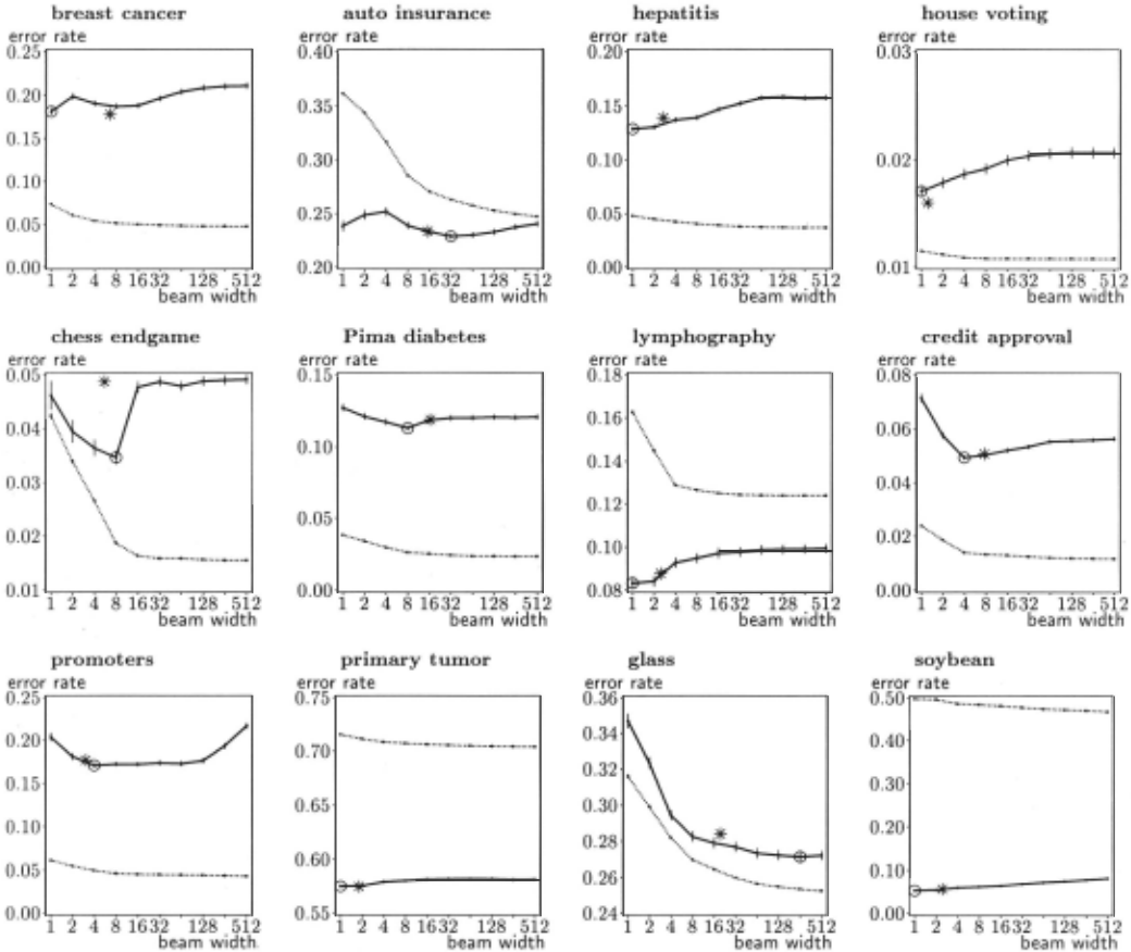
Results of these experiments appear in Figure 1 in which error rates are plotted against beam width. These er ror rates are weighted averages across the classes, the weights being the class relative frequencies in the train ing set. The dotted lines in each graph show the aver age £ values of the rules selected; without exception, £ values decline with beam width as more extensive search discovers rules with lower predicted error rates. The solid lines, however, show the average true error rate of the rules as measured on the unseen test data. (The vertical bars show one standard error either side of the mean; the open circles flag the beam correspond ing to the lowest true error rate; and the asterisks are explained in the next section.) As can be seen, the be havior of the true error rate is quite unlike that of the estimated rate .C. With some datasets such as the pro moter domain, increasing search first lowers the true er ror rate, then causes it to rise, an example of the same non-monotonicity observed by Rymon [1993]. On other domains such as hepatitis, more extensive search is uni formly counter-productive. Only for the glass dataset does the true error rate of the selected rule decline near monotonically with increased search.
To understand what is going on, we examine in more detail the chess endgame dataset, a particularly striking example of non-monotonicity. Separating results for the two classes (Figure 2), we can see that good rules for the majority class are found from the complete dataset with relatively small beam widths and thereafter improvement is slight. The U shape of the curve is due to the minority class, for which a marked change occurs at beam width 16.
In one typical trial, search at beam width 8 finds a con junction of three tests (RI) that is satisfied by 18 items of the minority class and none of the other class. Fur ther specialization of R1 can only decrease its cover and hence its £ value. However, there is also a conjunction of five tests (R2) that covers 32 items of the minority class and 7 items of the other class. Now, in order to discover a rule with left-hand side T1 and T2 and ... and Tn, the beam at level i must contain at least one conjunction of i of these tests, for all values of i from 1 to n-1. Conjunct R2 is difficult to find because no single test or pair of tests has a low £ value. For this trial, the £ value of the best single test ranks sixth among all single tests, so R2 is eliminated unless the beam width is at least 6. The best combination of two of the five tests has an £ value that ranks thirteenth among all two-test combinations, so the beam width needs to be at least 13 if R2 is not to be eliminated at the second level of the beam search. Once it is found, however, the large number of attributes in this domain allows R2 to be refined by the addition of seven further tests, giving a rule R3 that covers 30 items without error. In terms of the £ measure, R3 has a lower predicted error than R1 and so is preferred.
When evaluated on the test data, however, the com plex rule R3 misclassifies five items of the 31 that it matches, approximately the same error rate as the con junct R2 from which it was derived. On the other hand, the rule R1 is more accurate, misclassifying one of the thirteen items that it covers. Increasing the beam width from 8 to 16 allows the "fluke" R3 to be discovered, with a consequent increase in the error rate.
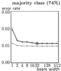
minority class (26%)
error rate
0.20
:::~
0. 05
..... \ .. .
..... ······-
····-····-····-····-·····
o.oo 1 2 4 8 1632 128 512
beam width
Figure 2: Chess endgame showing individual classes
3 Selecting a Beam Width
Having established that extensive search can lead to less accurate rules, we now discuss a method for limiting search.
For the domains of Figure 1, the most accurate rule is often found with a beam width w greater than 1 (where w=1 corresponds to greedy search) but less than 512, taken here as an approximation to exhaustive search. Suppose now that a layered search were conducted by starting with w=1 and doubling the beam width at each iteration. Could we select the appropriate beam width so as to obtain the most accurate rule? This decision clearly cannot be made with reference to the £ value alone, since this always decreases with further search.
The following probabilistic argument was inspired by the famous Occam paper [Blumer, Ehrenfeucht, Haus sler, and Warmuth, 1987). If the true error rate of a rule is r, the probability that the rule will give no more than e errors in n trials is given by
If there are h rules, all having an error rate of r or more, the probability that any one of them will give e or less errors inn trials is at most h x P(n,e,r) whether or not the rules are independent .
Now, let hw denote the number of rules examined dur ing the search with beam width w and let rw satisfy
If all these rules had error rate greater than or equal to rw, there would be up to an even chance that one of them would give no more than ew errors in nw trials. We use this value of rw as a guesstimate of the accuracy of the best rule selected from the hw candidates. As w takes on the values 1,2,4, ... , the corresponding values of hw, nw and ew can be determined and the value of r w computed. We take the overall best rule to be that for which rw is minimal.
There are numerous over-simplifications in this argu ment. For instance, it ignores the effect of beam selection at each level; search for the rule with minimal £ value is guided by the £ values of partial rules, so that the
| Beam Width | Items Covered | Rules Examined | Computed Estimate | |
|---|---|---|---|---|
| w | ew | nw | h w | Tw |
| 1 | 0 | 10 | 168 | 0.441 |
| 2 | 0 | 17 | 330 | 0.317 |
| 4 | 0 | 21 | 699 | 0.292 |
| 8 | 0 | 21 | 1265 | 0.311 |
| 16 | 0 | 23 | 2771 | 0.313 |
| 32 | 0 | 23 | 4758 | 0.329 |
| 64 | 0 | 23 | 7358 | 0.341 |
| 128 | 0 | 23 | 11768 | 0.354 |
| 256 | 0 | 23 | 17417 | 0.365 |
| 512 | 0 | 23 | 24902 | 0.375 |
"ew errors in nw trials" is not a fair experiment. Again, "number of rules examined" is an imprecise concept - many putative rules cover no examples, and some rules are pruned as described in Section 2. For these exper iments, hw is taken as the number of distinct attribute combinations considered during search on the basis that , for each such combination, there will be some test on ev ery selected attribute that minimizes the rule's £ value.
Table 2 illustrates the values for the positive class of the promoters dataset in one trial. Greedy search finds a rule that covers 10 items without error. Increasing the beam width to 2 causes a larger number of rules to be examined but yields a better rule covering 17 items; still better rules are found at beam widths 4 and 16. In the latter case, the number of rules examined increases the chance that the rule is a fluke, as reflected by its higher rw value. The rule encountered at beam width w=4 is consequently chosen as the overall best.
We can now explain the asterisks in Figure 1. At each trial, and for each class, a best beam width is selected as above using only the training data. The asterisk indi cates the average beam width selected and the average of the corresponding error rates on the unseen test data. 1 With the notable exceptions of the chess endgame and glass datasets, the average beam widths chosen are near the lowest points on the curves, providing some empirical support for the beam width selection strategy.
4 Learning Complete Classifiers
The search for individual rules can be extended to learn complete classifiers using the standard covering method [Michalski, 1980):
For each class Cx in turn: Mark all items of class Cx as uncovered. While uncovered items of class Cx remain: Find and retain the best rule. Mark as covered all class Cx items that
satisfy the rule.
1 The asterisk will not normally lie on the solid curve be cause the beam width selected varies from class to class and from trial to trial.
breast cancer
house voting
lymphography
primary tumor
auto insurance
chess endgame
credit approval
glass
hepatitis
Pima diabetes
promoters
soybean
Ratio to LS
| Error Rate (%) | Number of Rules | Theory Size | Time (sees) | ||||||||
|---|---|---|---|---|---|---|---|---|---|---|---|
| GS | LS | ES | GS | LS | ES | GS | LS | ES | GS | LS | ES |
| 28.8 | 28.8 | 29.1 | 43.0 | 29.4 | 26.0 | 132.9 | 106.4 | 101.2 | 0.1 | 1.5 | 13.4 |
| 5.7 | 5.6 | 5.7 | 14.3 | 10.9 | 10.1 | 37.5 | 31.7 | 30.3 | 0.1 | 0.4 | 11.1 |
| 22.1 | 18.9 | 19.0 | 14.4 | 10.4 | 9.5 | 33.6 | 30.1 | 30.1 | 0.0 | 0.2 | 6.5 |
| 58.3 | 58.5 | 58.3 | 59.8 | 53.3 | 45.9 | 269.5 | 256.0 | 234.6 | 0.2 | 2.0 | 54.4 |
| 31.4 | 31.1 | 31.4 | 33.4 | 18.7 | 14.2 | 70.1 | 57.5 | 58.6 | 0.2 | 2.7 | 25 .8 |
| 10.7 | 10.3 | 10.4 | 44.0 | 28.9 | 27.3 | 130.7 | 112.2 | 113.7 | 0.3 | 4.7 | 150.9 |
| 16.7 | 16.4 | 16.4 | 58.5 | 31.7 | 25.0 | 161.9 | 120.9 | 118.1 | 0.4 | 10.2 | 64.6 |
| 36.2 | 34.1 | 33.2 | 27.3 | 18.1 | 15.6 | 74.2 | 59.8 | 56.5 | 0.1 | 1.1 | 8.0 |
| 18.1 | 19.1 | 20.0 | 14.3 | 10.4 | 9.4 | 29.7 | 27.0 | 27.9 | 0.1 | 0.3 | 1.9 |
| 25.9 | 26.9 | 27.2 | 96.3 | 50.1 | 44.3 | 301.2 | 207.4 | 208.7 | 0.8 | 14.8 | 34.1 |
| 27.4 | 24.6 | 28.8 | 8.3 | 5.5 | 4.1 | 16.4 | 13.5 | 14.1 | 0.0 | 0.2 | 4.2 |
| 11.7 | 12.4 | 13.0 | 39.4 | 35.9 | 29.5 | 112.4 | 108.9 | 106.6 | 0.4 | 2.4 | 67.3 |
| 1.023 | 1.000 | 1.024 | 1.486 | 1.000 | 0.857 | 1.197 | 1.000 | 0.987 | 0.10 | 1.00 | 17.40 |
When determining the best rule above, only uncovered items of class Cx and all items of other classes are con sidered. Whereas Webb [1993] finds the rule with the guaranteed lowest C value at each iteration, we use the best rule encountered by three kinds of heuristic search:
- GS: Greedy search with beam width w=l.
- LS: Layered search with beam widths w=1, 2, 4, 8 and so on to a maximum of 512. For each beam width, the rule with lowest C value encountered during search is retained and its rw value determined, the overall best rule being the one of these with lowest rw . The layered search is terminated whenever two successive values of w fail to improve on the best value of rw found so far.
- ES: Extensive search with fixed beam width w=512, again taken to approximate exhaustive search.
An unseen item is classified by the ruleset by finding the rule with lowest C value that matches it, then assigning the item to the class specified in that rule's right-hand side. An item that satisfies no rule is assigned the most frequent class observed in the training set.
The experimental design was similar to that described in Section 2: for each dataset, 500 trials were conducted, splitting the data into stratified equal-sized training and test sets. Three classifiers were constructed from the training set using greedy (GS), layered (LS), and exten sive (ES) search, respectively, and each classifier evalu ated on the test set. Results averaged over the 500 rep etitions appear in Table 3. A simple indicator of theory complexity is provided by theory size, the total number of tests in all rules. Times are for a DEC AXP 3000/800 workstation.
Those error rates for GS and ES shown in bold face are significantly 2 different from LS. Layered search is sig nificantly better than greedy search in five domains and worse in three. When compared with extensive search, layered search is significantly better in six domains and worse in only one. Over the 6000 trials, LS is better than GS in 2822 trials and worse in 2534, while it is better than ES in 2927 trials and worse in 2438; both results are significant at better than p=O.OOOl.
2 Two-tailed sign test, p=0.05.
The ratio to LS figures in the final row give an overview across the twelve domains; each is the aver age ratio of a result to that for layered search. For these datasets, the theories found using LS have less than 98% of the error of those produced by either greedy or exten sive search. LS requires 10 times as much computation as GS, but the absolute difference is small since the lat ter is so economical. Extensive search (where w is fixed at 512) is 170 times slower than greedy search and 17 times slower than layered search, even though the latter requires repeated search with increasing beam widths.
5 Theory Complexity and Search
Discussion of the chess endgame example in Section 2 might suggest that this problem is just another instance of overfitting - extensive search is leading to the con struction of elaborate rules. Existing mechanisms for overfitting avoidance, such as Rissanen's Minimum De scription Principle [Quinlan and Rivest, 1989; Cameron Jones, 1992], might thus be sufficient to prevent the choice of rules with low predictive accuracy. We offer two arguments against this hypothesis.
As can be seen in Table 3, ranking the search methods by the complexity of the theory produced does not cor relate well with the accuracy of the theories. Although ES often finds more complex individual rules, this com plexity is counterbalanced by their increased coverage. Extensive search results in complete theories that are simpler than those found by layered search, and much simpler (20%) than those produced with greedy search. Yet, on average, the ES theories are less accurate than their LS counterparts and have similar accuracy to the GS theories.
The second is empirical, based on preliminary ex periments that assess the impact of oversearching on instance-based learning. For these trials, a classifier con sists of a subset of the training items, with an unseen item assigned to the class of the most similar retained item. All classifiers for a domain are constrained to consist of exactly the same number m of retained items, so that all theories have identical complexity. Beam searches of various widths are again carried out, this time to find the m items that give the lowest classifi cation error on the training set. Results with the same twelve datasets are reminiscent of Figure 1: increased search leads to better and better sets of retained items as assessed on the training data, but the classifier's perfor mance on unseen test data exhibits either a continuous decline or aU-shaped curve in six of the twelve domains.
6 Conclusion
This paper provides further evidence that more search does not necessarily result in better learned theories. In most of the domains studied here, expanding search leads eventually to a decline in predictive accuracy as idiosyncrasies of the training set are uncovered and ex ploited. This phenomenon of oversearching has also been observed in other domains and, indeed, with at least one other heuristic criterion. 3
For the twelve datasets reported here, an iterative lay ered search with beam width limited by a probabilistic criterion r w was found to have better overall performance than either greedy or extensive search. Even so, the ar gument that underpins the derivation of the rw value, and thereby selection of the "best" beam width, is sim plistic and we are confident that a better criterion can be developed.
We believe that oversearching cannot be controlled by complexity-based mechanisms such as the MDL prin ciple; the disadvantages of oversearching seem to be somehow orthogonal to problems of overfitting. MDL is rightly popular because it provides a well-justified frame work for mapping apparent accuracy and theory com plexity into a uniform measure based on coding length. Ideally, we would like to see oversearching dealt with in a similarly clean manner by the development of a single metric that embodies all three factors: accuracy, theory complexity, and extent of search.
Acknowledgements
We are grateful to Pat Langley for his detailed and help ful comments on a draft ofthis paper, and to the anony mous reviewers who suggested both improvements and areas for further research. The breast cancer, lymphog raphy and primary tumor datasets were provided by the Ljubljana Oncology Institute, Slovenia. Thanks to the UCI Repository and to its maintainers, Patrick Murphy and David Aha, for providing access to the datasets used here.
3 1n place of the Laplace estimate, we have also tried a confidence limit function UcF [Quinlan, 1993, page 41]. This function turns out to be even more susceptible to coincidences in the training data; a majority of the domains discussed here show a monotonic decrease in predictive accuracy with increased beam width.
@inproceedings{ijcai1995p132,
  title     = {Oversearching and Layered Search in Empirical Learning},
  author    = {Quinlan, J. Ross and Cameron-Jones, R. Mike},
  booktitle = {Proceedings of the Fourteenth International Joint Conference on
               Artificial Intelligence, {IJCAI-95}},
  publisher = {International Joint Conferences on Artificial Intelligence},
  editor    = {Chris S. Mellish},
  pages     = {1019--1023},
  year      = {1995},
  note      = {Learning},
  url       = {https://ijcai.org/proceedings/1995/132},
}
TY - CPAPER TI - Oversearching and Layered Search in Empirical Learning AU - Quinlan, J. Ross AU - Cameron-Jones, R. Mike T2 - Proceedings of the Fourteenth International Joint Conference on Artificial Intelligence, IJCAI-95 PB - International Joint Conferences on Artificial Intelligence PY - 1995 SP - 1019 EP - 1023 UR - https://ijcai.org/proceedings/1995/132 ER -Copied
Machine-readable versions of this paper, for tools and AI agents:





