
Qualitative Analysis of Causal Graphs with Equilibrium Type-Transition
Proceedings of the Fifteenth International Joint Conference on Artificial Intelligence. Diagnosis and Qualitative Reasoning. Pages 542-547.
© 1997 International Joint Conferences on Artificial Intelligence
Abstract
In this paper, we present a method to qualitatively compute the global characteristics of causal graphs by the analysis of the underlying dynamical systems, rather than traditional qualitative simulations which suffer from intractability and difficulty in understanding their simulation results. The key idea is to translate a given causal graph into an autonomous dynamical system and to analyze equilibrium points in the system. The method requires no numerical information and it has the advantage of computing the conditions under which a certain equilibrium type holds and when equilibrium type-transitions occur. The method is firmly based on mathematical grounds, and the result is guaranteed to be valid for linear systems under the specified conditions.
- [Chatelin, 1988] F. Chatelin. Valeurs propres de matrices (in French) . Masson (Paris) , 1988.
- [Clancy and Kuipers, 1992] D. J. Clancy and B. J . Kuipers. Aggregating behaviors and tractable simu- lation. In AAAI Design from Physical Principles Fall Symposium Working Notes, pages 38-43, 1992.
- [Crawford et al., 1990] J. Crawford, A. Farquhar, and B. J. Kuipers. QPC: A compiler from physical mod- els into qualitative differential equations. In Proc. of AAAI-90, pages 365-372, 1990.
- [De Mori and Prager, 1989] R. De Mori and R. Prager. Perturbation analysis with qualitative models. In Proc. of IJCAI-89, pages 1180-1186, 1989. IJCAI
- [Forbus, 1984] K. D. Forbus. Qualitative process theory. Artificial Intelligence, 24:85-168, 1984.
- [Fouche and Kuipers, 1992] P. Fouche and B. J. Kuipers. Reasoning about en- ergy in qualitative simulation. In IEEE Transactions on Systems, Man and Cybernetics 22, pages 47-63, 1992.
- [Guckenheimer and Holmes, 1990] John Guckenheimer and Philip Holmes. Nonlinear Oscillations, Dynam- ical Systems, and Bifurcations of Vector Fields ( Ap- plied Mathematical Sciences Vol. 42 ). Springer-Verlag, 1990.
- [Ishida, 1989] Y. Ishida. Using global properties for qualitative reasoning: A qualitative system theory. In Proc. of IJCAI-89, pages 1174-1179, 1989. IJCAI
- [Iwasaki and Bhandari, 1988] Y. Iwasaki and I. Bhan- dari. Formal basis for commonsense abstraction of dynamic systems. In Proc. of AAAI-88, pages 307- 312, 1988.
- [Kuipers, 1986] B. J. Kuipers. Qualitative simulation. Artificial Intelligence, 29(3) :289-338, 1986.
- [Kurumatani and Nakamura, 1996] K. Kurumatani and M. Nakamura. Generating qualitative equations about macro-behaviors of foraging in ant colony. In Proc. of German Conference on Bioinformatics, GCB'96 (Leipzig), pages 142-147, 1996.
- [Kurumatani, 1995] K. Kurumatani. Generating causal networks for mobile multi-agent systems with qualita- tive regions. In Proc. of IJCAI-95, pages 1750-1756, 1995. IJCAI
- [Lee and Kuipers, 1993] W . Lee and B. J. Kuipers. A qualitative method to construct phase portraits. In Proc. of AAAI-93, pages 614-619, 1993.
- [Nakamura and Kurumatani, 1996] M. Nakamura and K. Kurumatani. Formation mechanism of pheromone pattern and control of foraging behavior in an ant colony model. In Proc. of Fifth Int'l Conf. on Ar- tificial Life, ALife V (Nara), pages 48-56, 1996. 548 DIAGNOSIS AND QUALITATIVE REASONING [Nishida and Doshita, 1991]
- T. Nishida and S. Poshita. A geometric approach to total envisioning. In Proc. of IJCAI'91, pages 1150-1155, 1991. IJCAI
- [Rose and Kramer, 1991] P. Rose and M. Kramer. Qual- itative analysis of causal feedback. In Proc. of AAAI- 91, pages 817-823, 1991.
- [Sacks, 1987] E. Sacks. Piecewise linear reasoning. In Proc. of AAAI-87, pages 655-659, 1987.
- [Weld, 1987] D. S. Weld. Comparative analysis. In Proc. of IJCAI-87, pages 959-965, 1987.
- [Yip, 1988] K. Yip. Generating global behaviors using deep knowledge of local dynamics. In Proc. of AAAI- 88, pages 280-285, 1988.
- [Zhao, 1994] F. Zhao. Extracting and representing qual- itative behaviors of complex systems in phase space. Artificial Intelligence , 69:51-92, 1994.
References were extracted automatically from the PDF and may contain errors.
Full text extracted automatically from the PDF; figures, tables and equations may differ. The PDF is the version of record.
1 Introduction
Traditional qualitative simulation methods are based on the qualitative value representation for each state vari able. The behaviors of a target system are simulated on this discrete quantity, and the methods cannot avoid the ambiguity and intractability in their results.
In this paper, we present a qualitative method to an alyze the global characteristics of a target system de scribed as a causal graph without qualitative simula tions, based on dynamical systems theory.
The key idea of the method is 1) to prepare a target system in the notation of autonomous linear dynamical system, 2) to analyze the type of equilibrium points, and 3) to determine the conditions when equilibrium type transitions occur.
The method requires no numerical information. In addition to it, the method has the advantage of com puting the conditions under which a certain equilibrium type holds and when equilibrium type-transitions occur. This kind of reasoning ability has not been achieved by previous works in the literature.
After the basic introduction of dynamical systems theory (section 2), we will analyze the basic simply-
Mari Nakamura
LERC, Electrotechnical Laboratory Nakoji 3-11-46, Amagasaki, Hyogo 661, Japan
mari@osaka.etl.go.jp
connected loops (section 3), followed by the key com ponents of our method (section 4, 5, 6) and examples to show the ability of the method (section 7).
2 Basic Characteristics of Dynamical Systems
Linear dynamical systems are expressed by a differential equation:
Each element of x = (xi, x2 , ... , xn)t is a state variable, and the vector x is called state vector 1 .
Equation (1) represents a linear dynamical system, which has one trivial equilibrium point x = 0 and pos sibly has non-trivial ones.
Non-linear dynamical systems are represented by a dif ferential equation:
Possibly there exist several equilibrium points given by f( x) = 0. The behavior in the neighborhood of an equi librium point x 0 is precisely governed by a linear equa tion:
Computing the Jacobian matrix J can be done automat ically by symbolic differentiation.
Equilibrium points are classified into attractor, repel lor or saddle. Trajectories approaching to an attractor will finally reach the point. From a repellor, trajecto ries start and never return to the point. Trajectories approaching to a saddle are first attracted but finally repelled by the point.
The characteristics of an equilibrium point can be specified by the eigenvalues of the coefficient matrix (Ta ble 1). In general, the eigenvalues consist of 1) real num bers and 2) pairs of conjugate complex numbers. If all the real parts of eigenvalues are positive or negative, the point is a repellor or an attractor respectively. Other wise, the point is a saddle which is a combination of repellor and attractor. Exceptions are the cases where the real parts of some eigenvalues are zero. Such a point is called non-hyperbolic.
1 Throughout the paper, (x1, x2, . .. , Xn) 1 represents n tuple column vector.
| Eigenvalue: .A=a±bi | Real Number: b=O | A Pair of Conjugate Complex: b =f:. 0 |
| a>O | nodal repellor | spiral repellor |
| a=O | zero-eigenvalue | center |
| a<O | nodal attractor | spiral attractor |
About non-hyperbolic point [Guckenheimer and Holmes, 1990], if it is a pair of purely imaginary numbers, it is called center, which has eternal periodic trajectories around the point.
The eigenvalue whose value is exactly zero is called zero-eigenvalue. If there exist zero-eigenvalues, the be haviors around the point become strange ones. We ig nore this special case for a while, before addressing struc tural stability in section 5.
3 Analysis of Causal Loops
In this section, we analyze basic simple loops connected by influence relations, i.e., causal loops with time-delay.
3.1 Illustrative Example
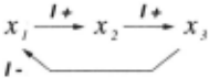
An example is a simple loop of three variables connected by direct influence relations [Forbus, 1984] (Figure 1). It is described by an equation:
where a21, a32 > 0 and a13 < 0.
Propagation-based qualitative simulation methods cannot be applied to this kind of example with loops, because a propagation will go back to its starting point.
The constraint-based filtering method, i.e., QSIM [Kuipers, 1986], can predict the behavior of the system. Starting with an initial state, e.g.,
the method produces the unique successors and finds out that the twelfth state is qualitatively equivalent to the initial one, i.e., the behavior is cyclic, then stops.
There is basically no way to know which type of behavior it is (spiral attractor, repellor, or center) by QSIM. Although the energy filter [Fouche and Kuipers, 1992] and the envisionment-guided simulation [Clancy and Kuipers, 1992] have been proposed for that purpose, they have restrictions in applicability, e.g., the dimension of the state space.
Actually, this equilibrium point is a saddle which consists of a one-dimensional attractor and a two dimensional spiral rep ell or, whenever a21, a32 > 0 and a 13 < 0. The trajectory will be repelled with rotating around the equilibrium point.
We will show a method of extracting these global char acteristics of the system by qualitatively analyzing equi librium points, instead of carrying out qualitative simu lations.
3.2 Qualitative Analysis of Simple Loops
The general form of simple loops connected by direct influences are described by an equation:
The loop shown in Figure 1 is an instance (n = 3) ofthis class.
Definition 1
The loop constant of a loop by Equation (3) is defined as L = a 1 n a21 ... an n-I· The loop constant should not be zero by definition. I
Definition 2
A loop is called positive or negative, iff its loop constant is greater or less than zero, respectively. I
The following lemma tells the relation between the eigenvalues and the trace of a matrix.
Lemma 1 (Eigenvalues and Trace)
The summation of the eigenvalues Ai of a matrix A is equal to the trace Tr(A) = L:~1 a;;, i.e.,
Proof:
Eigenvalues are given by an equation:
By comparing the equation with the eigenpolynomial,
where Tr(A) is the trace and Det(A) is the determinant, the proposition holds. I
Consequently, the summation of the real parts of all eigenvalues is also equal to the trace.
We can conclude the characteristics of simple loops with time-delay as follows.
Theorem 1 (Characteristics of Simple Loops)
The equilibrium point of a simple loop described by Equation (3) is a saddle when n ~ 3, except:
- The neighborhood of the equilibrium point of a pos itive loop includes a center as its subspace, iff both n and nl2 are even numbers, e.g., n = 4, 8, 12, ....
- The neighborhood of the equilibrium point of a neg ative loop includes a center as its subspace, iff n is even and nl2 is odd, e.g., n = 6, 10, 14, ....
Proof:
The eigenvalues are given by an equation An - L = 0, where Lis the loop constant. Obviously, zero-eigenvalue is not a solution. Since the trace is zero, the sum of the real parts of all eigenvalues is zero. Assume that the loop is positive, i.e., L > 0. Since one eigenvalue is a positive real number p i n, there should exist at least one eigenvalue whose real part is negative. Consequently, the point is a saddle except the case where there exists a pair of purely imaginary eigenvalues A = ± L 1 1ni (a center). All conditions for this case are limited to excep tions shown above. Similarly the theorem holds when the loop is negative. I
This theorem tells that simply-connected causal loops should become a saddle when its length is greater than or equal to three, i.e., trajectories are first attracted to the equilibrium point but finally they are sure to move to the infinity point. The direction of the repelling move must include ( +, +, ... , + )t when the loop is positive.
The exceptional case about a center does not have the importance from the actual application point of view, because only a very little perturbation will make it be come a spiral at tractor or repellor (in section 5).
Special cases in lower dimensions are as follows.
Theorem 2
A loop of length one is called self-feedback. A positive self-feedback has a repellor as its equilibrium point , and a negative self-feedback has an attractor.
A loop oflength two is called mutual-feedback . A positive mutual-feedback has a saddle, and a negative mutual feedback has a center. I
4 Convergence of General Systems
From the engineering point of view, the system is called convergent (or stable) when the equilibrium point is an attractor, because all the state variables, and conse quently the system itself, are sure to converge on a stable state (the equilibrium point) .
In this section, we discuss a method of verifying the convergence of general systems given by Equation (1).
4.1 System of Short Loops
The first way is to check whether a system consists of short loops whose lengths are less than three. It is straightforward to obtain the following theorem from the result in the previous section.
Theorem 3 (Convergence of Short Loops)
A system satisfying the following conditions is conver gent, i.e., it has an attractor as its equilibrium point, while possibly the neighborhood includes a center.
- There exists no positive self-feedback, and there ex ists at least one negative self-feedback.
- There exists no positive mutual-feedback.
- There exists no loop whose length is greater than or equal to three. I
The conditions are same in essence as the results ob tained by Ishida [Ishida, 1989].
The conditions required in this theorem are too strict to apply them to real systems, because many systems have loops whose lengths are greater than two.
4.2 System with Self-Feedbacks
The second way is to check whether each variable in the system has 'enough' self-feedbacks. This technique can be applied not only to short loops, but also to general complex systems.
The method is based on the relations between eigen values and diagonal elements in a matrix, proven in lin ear algebra [Chatelin, 1988].
Definition 3 ( Gershgorin Circle)
For a matrix A E Rnxn, A = (ai j ), the Gershgorin circle in a complex plane for the i-th diagonal element a ii is defined as:
I
The center of the i-th Gershgorin circle in a complex plane is the place of the i-th diagonal element, and the radius is the summation of the elements in the i-th row. About the relations between the Gershgorin circles and the places where eigenvalues exist, the following theorem holds.
Theorem 4 (Gershgorin Circle and Eigenvalue) Any eigenvalue of A E Rn x n exists in (at least) one of the Gershgorin circles of A. I
This theorem tells that any eigenvalue exists in the area covered by Gershgorin circles, which can be used to reason about the type of equilibrium.
The condition for the convergence of a target system is given by the following theorem.
Theorem 5 (Convergence by Self-Feedbacks)
If all the diagonal elements are small enough, i.e., each state variable has enough negative self-feedback, the sys tem is convergent. The condition is:
Similarly, the point becomes a repellor, when:
By this theorem, if all diagonal elements are smaller than the sum of other elements' absolute values in the same row, the system is convergent .
Intuitively speaking, it is rare for a complex system to become convergent, unless we add some special mecha nisms to the system. The theorem shows such a mecha nism which surely makes the system convergent.
5 Structural Stability and Equilibrium Type-Transition
Imagine a situation where we add a little perturbation to the vector field of a target system, i.e., to the elements of the coefficient matrix A in Equation ( 1). The type of the equilibrium point (attractor, repellor, or saddle) will not change by the perturbation if its value is small enough. This attribute is called structural stability of the system [Guckenheimer and Holmes, 1990].
However, a system is structurally 'unstable' when it has a non-hyperbolic equilibrium point, i.e., the real parts of some or all eigenvalues are zero. Such a point is sure to transit to another type of equilibrium regardless of the value of a perturbation, because the real parts of eigenvalues are sure to become positive or negative.
The manner of 'type-transition' of a non-hyperbolic equilibrium point by a perturbation is as follows.
Center to Spiral Repellor or Attractor
A pair of purely imaginary numbers will change into a pair of conjugate complex numbers whose real part is positive or negative. Thus a center will transit to a spiral repellor or attractor by a perturbation.
Zero-Eigenvalue
If there exists only one eigenvalue which is exactly zero, i.e., zero-eigenvalue, the determinant of A is zero by the eigenpolynomial of Equation ( 4). In this case, the rank of A is n- 1 and there exists a non-trivial solution of A = 0, which means that there exists a equilibrium hyperline in the phase space. The equilibrium line will change into a nodal repellor or attractor by a perturba tion regardless of its value.
In order to determine the existence of a zero eigenvalue, we have to compute the rank of A, e.g., to count the number of linearly independent rows or columns of A. Because we assume that A is qualita tive, i.e., the exact values of the elements of A are not given, zero-eigenvalues exist only for specific sets of the numeric values. Consequently only the possibility of the existence can be pointed out. In special cases, however, we can show that a target system has zero-eigenvalues only by qualitative computation.
If there exist more than one zero-eigenvalues, it is usu ally very difficult to handle the equilibrium point and the behavior of the total system. We will not address this kind of points for simplicity.
6 Transforming General Graphs Including Monotonic Relations
Before applying our method to exaii?-ples, we address the relations called indirect influences or monotonic re lations, which are constraints on the manner of variable value change; and show a way of transforming general graphs which include such relations into Equation (1).
We express indirect influence Q+ [Forbus, 1984] by monotonic relation M+ defined in [Crawford et al., 1990]:
A monotonic relation y = M{i(x) puts another con straint "x = 0 => y = 0" in addition to (6).
In order to decide n in Equation (6), i.e., to decide how many variables Xi indirectly influence y, we have to count the arcs flowing into y.
An arbitrary combination of monotonic relations in a causal graph can be mathematically meaningless. We assume that the condition for the change of variables concerning partial differentiation holds in a given causal graph, i.e., there is no loop which consists of monotonic relations. The exception is a simple monotonic loop whose all nodes have only one source, i.e., n = 1 in Equation (6) for all the nodes in the loop.
On this assumption, we can transform a given causal graph into a simpler form which can be handled by our method, using the following transformation rules.
Transitive and Distributive Law
The notation 'EEl ' means qualitative addition while '+' means exact addition. Similar relations hold for the com binations of M- , - and e.
Variable Identification by Monotonic Relations
When a monotonic relation y = M+(x) exists, we can identify a variable x as y, with regard to the direction of variable change, i.e., the sign of time-derivate, iff there exists no other monotonic relation flowing into y, i.e.,
where M is any of M+, M-, M{i, or M 0 -. Similarly, two variables connected by M- can be identified iff (9) holds, although the direction of change is opposite.
Two variables connected by M{i or M 0 - can be identi fied as a same qualitative variable in { +, 0,-}, although both the direction of change and the value are opposite in the case of M 0 -.
Loop Including Monotonic Relations
The important issue is a loop which consists of both (direct) influences and monotonic relations. If there is no monotonic relation in the loop after variable identi fication by monotonic relations, the loop is handled in the way discussed in the previous sections. In this case, the sign of loop constant should be changed according to the number of monotonic relations M-, M0 appearing in the original loop.
When we cannot eliminate all monotonic relations in a loop, the behavior of the loop is separated into cases de pending on the status of variables flowing into the loop.
7 Applications
We have applied our method to examples in the litera ture and found that many of the examples have small numbers of state variables in essence, e.g., from one to three variables. The method captures the characteristics of this class of the systems in lower dimensions which qualitative simulations can handle with less difficulty. In this section, we address three examples to show the ability of our method.
7.1 U-Tube
The first example is U-tube [Crawford et al., 1990] . Two tanks A and B are connected by a liquid flow path at the bottom of them 2 . In the initial state, tank A is filled with water and tank B is empty.
The system has six state variables (pressure at the bottom of tank Pa, Pb ; mass in tank ma, mb ; flow rate r ; pressure difference Pd)· The causal graph of the system is as follows.
After applying variable-identification rules, we obtain the following qualitative equation which consists of only two variables Pa and Pb ( x = (Pa, Pb) t).
The outline of reasoning process about the behaviors of this system is as follows. Because the system has a positive loop of length two, the convergence of short loops does not hold (theorem 3). Although all eigenval ues exist in two circles which are placed in the negative half-plane, the circles also include the origin (0, o)t (theo rem 4). The convergence by self-feedbacks does not hold ~n the case where some eigenvalues exist on the origin, 1.e., they are zero-eigenvalues (theorem 5).
Actually, this system is a special one which has one zero-eigenvalue, since 1) the second row is equal to -a2/a1 times the first row (linearly dependent), 2) the number of linearly independent rows is 1, and conse quently, 3) the rank of A is 1.
Non-trivial solution of A= 0 is (k, k)t where k is an arbitrary real number, and the direction vector of equi librium line is (1, 1)t. Because the dimension is lower, di rect computation of another eigenvalue is possible. How ever, we can reason about it in a qualitative way, i.e., 1) another eigenvalue is a real number, but it is not zero because the rank of A is 1, 2) all eigenvalues exist in the negative half-plane, and consequently, 3) it should be a negative real number.
By these reasoning results, the phase space is obtained as shown in Figure 2 (a). From any initial point the trajectory will reach the equilibrium line and stop ~nit.
When a small perturbation is added to the system this equilibrium line will transit to a nodal repellor o; attractor. For instance, it will transit to a nodal attrac tor in Figure 2 (b), when a perturbation J1 > 0 J2 > 0 is added to A as follows. '
2 We ignore the portal which is included in the original problem to clarify the essential points.
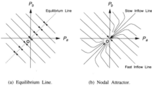
This perturbation physically means that a small leak ex ists in the liquid flow path. It is easy to know that both eigenvalues are negative real numbers. When the per turbation is relatively small, the trajectory will first ap proach the slow inflow line which the original equilibrium ~ine ab~ve has changed into, then move along the slow mflow hne, and finally reach the equilibrium point .
Relatively small perturbation in this case means that two negative eigenvalues have relatively different abso lute values. Iwasaki proposed a method to analyze the system which has relatively different eigenvalues [Iwasaki and Bhandari, 1988], although the method is valid only for an attractor and its main purpose is to decompose a large-scale system into sub-components.
This kind of 'equilibrium type-transition' discussed here cannot be reasoned by comparative analysis [Weld, 1987], nor perturbation analysis [De Mori and Prager, 1989] [Rose and Kramer, 1991], since these methods are valid for the position move of an equilibrium point within a certain equilibrium type.
In the original problem [Crawford et al., 1990], the flow rate is assumed to be equal to the pressure differ ence as. shown in Equation (10). This is the reason why the traJectory approaches the equilibrium state without oscillation. In real physical systems, however, the flow rate is not always equal to the pressure difference because of ~ner~ia of fluid and friction, which causes a damped osclllatwn before reaching the equilibrium state.
7.2 Damped Oscillation
~he second example is an oscillator governed by an equa twn:
Letting x1 = y, x2 = y, x following equation.
When f..L = 0, the system is an oscillator without damp. In this case, the system is a negative loop of length two, whose equilibrium type is center (theorem 2) . The tra jectory is a closed cycle around the origin (eternal peri odic oscillation).
Notice that two eigenvalues consist of a pair of con jugate purely imaginary numbers ± o: i, and that Tr(A) is zero. This non-hyperbolic equilibrium point changes its type into spiral attractor or repellor, when a little perturbation is added to the system.
When f-L > 0, the system is called damped oscillator. In such case, the eigenpolynomial (>. 2 +o: 2 ), which corre sponds to conjugate purely imaginary numbers, becomes (>. 2 + f-LA + o: 2 ), because the trace of A becomes -J.L. Con sequently, the real part of the eigenvalues becomes neg ative, i.e., the equilibrium type is spiral attractor. The trajectory approaches the origin while revolving around it.
7.3 Ant Colony's Macro-Behavior
The third example is a foraging behavior of an ant colony at macro-level [Kurumatani a~d Nakamura, 1996] [Ku rumatani, 1995]. It is a coordinated group behavior achieved by a simple behavior of individual ants with a communication method using chemical material.
The key mechanism of the system is that 1) an ant changes its behavior-mode according to the inter nal/external situation, 2) an ant which transports bait puts chemical material called trail on the ground, 3) the trail evaporates and becomes pheromone, and 4) diffused pheromone induces other ants to gather at the bait-place.
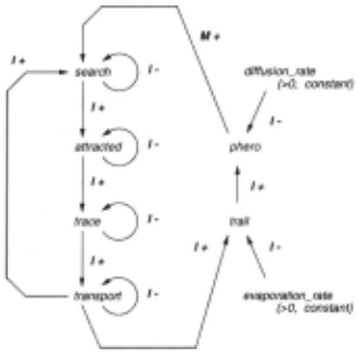
The system has the state variables for the number of ants in each mode and tjle amounts of trail and pheromone. The causal graph is shown in Figure 3.
There are two loops and six variables in the graph. Although four variables have self-feedbacks, the rest do not. The trajectory is sure to be repelled in the direction of ( +, +, ... , + )t, if influences on the variables phero and trail by other variables are greater than ones by two constants.
This system is purely qualitative one, because there is no way to know the exact numeric coefficients. Our method, however, captures the characteristics of the behavior which is empirically analyzed [Nakamura and Kurumatani, 1996], where the positive influence loop re ally works.
8 Non-Linearity in Causal Graphs
Our method is based on the characteristics of linear dy namical systems. It cannot be applied directly to general non-linear systems.
However, the results are valid for the systems de scribed by 'semi-linear' functions, e.g., influence, mono tonic, addition, and subtraction, since these semi-linear functions do not change the type of equilibrium and the characteristics of equilibrium neighborhood discussed in this paper can be extended globally to the whole phase space, although trajectories might be curved by non linearity of the functions . The examples in the previous section belong to this class.
It seems difficult to have purely qualitative methods of analyzing global topological characteristics of general non-linear systems. When a non-linear system is given, it is possible to qualitatively analyze each semi-linear seg ment of a phase space divided by piece-wise approxima tion and to connect them into a whole qualitative phase portrait. Methods in this direction of analyzing phase space [Sacks, 1987] [Yip, 1988] [Lee and Kuipers, 1993] and constructing the whole map [Nishida and Doshita, 1991] [Zhao, 1994] have been proposed. Applying our method in this direction is left for future work.
9 Conclusion
We have proposed a method to qualitatively analyze the characteristics of causal graphs without simulations.
The method consists of 1) pre-processing monotonic relations in a graph and reformulating it into a qual itative dynamical system, 2) analyzing the coefficient matrix and computing the type of equilibrium points, and 3) computing the conditions when equilibrium type transitions occur.
The method can be regarded as direct qualitative anal ysis of equilibrium points and their neighborhoods with out numerical information. It has the advantage of com puting the conditions under which a certain equilibrium type holds and when equilibrium type-transitions occur.
Future work includes applications of our theory to global topology analysis of non-linear systems and to automatic categorization of equilibrium type-transition in such systems.
Acknowledgement
A part of this work was carried out when the first author was staying at AI Lab. (LIA), Swiss Federal Institute of Technology, Lausanne (EPFL). We would like to thank Prof. Faltings and the members of LIA for fruitful dis cussions.
@inproceedings{ijcai1997p80,
  title     = {Qualitative Analysis of Causal Graphs with Equilibrium Type-Transition},
  author    = {Kurumatani, Koichi and Nakamura, Mari},
  booktitle = {Proceedings of the Fifteenth International Joint Conference on
               Artificial Intelligence, {IJCAI-97}},
  publisher = {International Joint Conferences on Artificial Intelligence},
  editor    = {Martha E. Pollack},
  pages     = {542--547},
  year      = {1997},
  note      = {Diagnosis and Qualitative Reasoning},
  url       = {https://ijcai.org/proceedings/1997/80},
}
TY - CPAPER TI - Qualitative Analysis of Causal Graphs with Equilibrium Type-Transition AU - Kurumatani, Koichi AU - Nakamura, Mari T2 - Proceedings of the Fifteenth International Joint Conference on Artificial Intelligence, IJCAI-97 PB - International Joint Conferences on Artificial Intelligence PY - 1997 SP - 542 EP - 547 UR - https://ijcai.org/proceedings/1997/80 ER -Copied
Machine-readable versions of this paper, for tools and AI agents:





