Using Global Properties for Qualitative Reasoning: A Qualitative System Theory

1 Introduction

Qualitative physics (de Kleer and Brown 1984] (or qualitative process theory (Forbus 1984]) has been stud­ ied recently. Qualitative reasoning is used for predicting and explaining the behavior of the physical system by using symbolic computation.

De Kleer and Brown (de Kleer and Brown 1984] use logical proof as the explanation for the physical behavior. They pointed out that the logical proof has undesir­ able features for making causal accouts, and proposed mythical causality. While their modeling is rather com­ ponent oriented, Forbus (Forbus 1984] developed pro­ cess oriented modeling. Kuipers' theory (Kuipers 1986] , however, starts from abstracting the mathematical model preserving qualitative information in the model. Both Kuipers (Kuipers 1986] , and de Kleer and Bo­ brow (de Kleer and Bobrow ·1984] developed simulation algorithms on their qualitative models. Both of them introduce higher order derivatives to predict change precisely._ The problems of these qualitative reasoning methods are:

1. Although these methods provide modeling perspec­ tives, they are not yet ready for the automatic or interactive generation of the qualitative models of large-scale systems such as industrial processing plants.
2. They do not use global properties which do not come from the local propagation of the constraint or state.

Falkenhainer and Forbus (Falkenhainer and Forbus 1988] focus on the problem of the modeling by considering the granularity of the model. We focus on the second problem using structural conditions for global properties. Struss (Struss 1988] and Lee and Kuipers (Lee and Kuipers 1988) also dis­ cuss the second problem with reference to the phase space portrait. We will present an alternative method for :filtering out spurious behavior using global proper­ ties, which can be checked on the graphically expressed qualitative model. The global properties of the system, such that an oscillation will converge on some point or not, can be discriminated to some extent by checking the sign structure of the graph. Our method seems to be more suitable for symbolic computation than with the method using geometric conditions, however ours suffers from the limitation that the target system must be linear.

Section 2 shows the qualitative model of dynamical systems. The qualitative model is a signed directed graph obtained by keeping the qualitative information of sign structures of a linear system. In section 3, global analyses such as stability analysis are made on the qual­ itative model.

2 Qualitative Model of a Dynanlical System

2.1 The qualitative model

Qualitative theory of linear systems, which has been studied extensively in econometrics [Quirk 1965, Quirk 1968] and mathematical ecology [Jefferies 1974], is used as a:n analysis tool for the qualitative model. In many systems such as chemical processing plants dy­ namical behavior is expressed or approximated by a linear differential equation:

(2-1) dxfdt =Ax, A E R"'x"'.

We use the qualitative model expressing the signed matrix A ·. 1 In the model, an arc is directed from node ito node j with the sign of (A.)ij· Most of the results of qualitative system theory are obtained for the state­ space expression of this linear system. Thus, in order to directly use this qualitative system theory, we transform the model into this state-space expression. All the in­ teractions whose phase lag are n > 1 are divided into n sequential interactions of phase lag 1 by introducing n-1 dummy variables (nodes). On the other hand, variables (nodes) connected by the interaction of phase lag 0 are regarded as one variable (node). In the global analysis of section 3, we assume the systems under discussion are already normalized.

Non-linear systems must be -first linearized in the fol­ lowing manner. Develop the system around the point of interest, then neglect the higher order non-linear terms. This linear approximation is only valid in the neigh­ borhood of the point. The linearized system must be expressed in state-space expression for later analysis.

Example 2.1

The model for the pressure regulator is shown below.

dXsfdt=-a·Po

dQifdt =b. (DP- c. Qi 2 I X s)

dPofdt = e · (Qo 2 - J ·Po)

1 Signed matrix A, of A is a triple value matrix defined as follows :

(A, )ij = +. ~, 0 if (A)ij > 0, < 0, = 0 respectively.

Xs area available for the flow

through the valve

Po pressure at outlet

Pi pressure at inlet

DP pressure drop across the valve

Qi inflow to the valve

Qo outflow from the valve

• a, b, c, e, f: appropriately chosen positive constants.

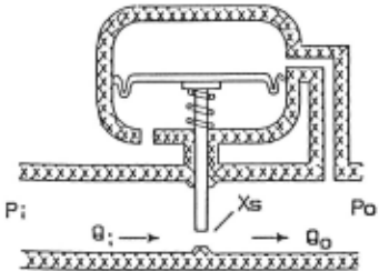
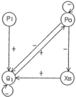
Fig. 1 shows a diagram of a pressure regulator. Fig. 2 is the signed digraph expressing t-he qualitative model. Since the phase lag of all the arcs is normalized to 1, only the sign is indicated in the arc.

2.2 Causality and system theoretic concepts

In dynamical system theory, many concepts such as ob­ servability and stability have been studied. Since these concepts have intuitive explanatory power, they may be used as aids for causal account. There seems to be an important relation between the concept of observability and causality. In system theory, observability is defined as:

"A system is sai9, to be observable by an ob­ server if it is possible to determine the initial state by observing the output signal from the observer during a :finite time starting from the initial time."

We can use the observability 2 (or its dual concept of controlability) as a tool to check the potential causabil­ ity. It is not against our intuition to say that the event dX =+(or-) can cause the event dY =+(or-) only when X is observable from Y.

3 Global Analysis

The main advantage of using state-space expression (21) of the qualitative model is that it allows many system theoretic analyses, especially the global analysis. This section presents several results which can be used as a tool for a global analysis on the qualitative model.

3.1 Qualitative stability analysis

A property of a system is called qualitative if it is de­ termined only by the sign structure of the qualitative model. In this section, we discuss the qualitative prop­ erty of the qualitative model. Two kinds of qualitative stabilities, and qualitative observability are defined as follows.

Definition 3.1. (sign stability and potential stability)

A qualitative model A, is called sign (potential) sta­ ble if all (some of) instances of the model are stable 3 · Definition 3.2. (sign observability)

The qualitative model with the observer is said to be sign observable if all instances of the model are observ­ able from the observer.

In the example 2.1, the graph indicates that the model can be decomposed into two strongly connected components 4 corresponding to the subsystem Pi and the subsystem consisting of Po, Q, Xs. Pi is observable from the subsystem of Po, Q, Xs and not in opposite way. Notice, however, that even if the model is decom­ posed into strongly connected components, the affecting subsystem may not be observable from the affected sub­ system in such cases that the affecting subsystem has a constant mode or two effects canceling each other. (Ob­ viously, the affected subsystem is not observable from the affecting subsystem.)

2 The observa.bility of the linear system ca.n be checked by a. matrix. Let y = Cx , y E Rlxm,c E Rnxm be ob­ served output of the linear system (2-1), then the observa.bil­ ity from y ca.n be known by testing whether or not the matrix (C, CA, CA 2 , .. . , CA"- 1 ] ha.ve the full ra.nk.

3 The solution of the system will asymptotically converge on a.n equilibrium point .

A necessary and sufficient condition for a qualitative model to be sign stable is obtained with the concept of sign observability.

Theorem 3.3.

A qualitative model is sign stable if and only if the qualitative model has the following properties.

(1) There is no positive loop 5 and there exists at least one negative loop,

1. there is no positive circuit of length two,
2. there is no circuit of length greater than two, and

( 4) by setting the subsystem of negative loops as observer, the rest of the subsystem is sign observable from the observer.

Proof

The conditions (1)-(3) guarantee that the system does not have ·divergent mode 6 · In order to further guaran­ tee that the system does has neither constant mode nor pure periodical modes we only have to put the condi­ tion that that the signals are always observable from the node having a negative loop. In other words, if the sys­ tem has pure periodical modes then the signal may not be observable by the cancellation of the oscillations of different phase. Likewise, if the system has a constant mode the signal is not observable.

Example 3.4.

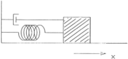
To demonstrate the power of the sign stability, let us consider the mass-spring system whose state-space expression is as below:

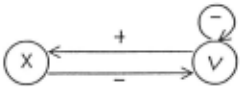
dX/dt = V

dVfdt = -kX- JV where k and f are positive con­ stants.

4 Strongly connected component is such subgra.ph tha.t for a.ll the pa.irs of nodes in the subgra.ph there exists a. pa.th from both sides.

5 A circuit is a. closed pa.th where the pa.th is a. graph connecting ma.ny nodes by a.rcs of the sa.me direction sequentia.lly. The sign of a. circuit is a. multiplication of a.ll the signs of the a.rcs included in the circuit. The length of the circuit is the number of a.ll the a.rcs included in the circuit. The circuit of length 1 is called a. loop.

6 For the system (2-1), divergent mode, pure periodical modes, a.nd constant mode a.re realized when the matrix A ha.s eigenvalues with positive rea.! pa.rt, pure imaginaries, a.nd 0 respectively.

Fig. 3 shows the diagram of a mass-spring system with dash pot. The qualitative model of the mass-spring system is shown in Fig. 4a. This system is known to be sign stable, since all the conditions of theorem 3.3 are satisfied. Thus, oscillation will always converge eventually. When f = 0 (when there is no loop at node V), however, the system is always in a pure periodical mode.

The necessary and sufficient conditions for a quali­ tative model to be potentially stable have not yet been obtained. We present some heuristics which will be used to identify the potentially stable sign structure.

Theorem 3.5.

A qualitative model is potentially stable if the sub­ graph of the the qualitative model is potentially stable.

Proof

One of the powerful heuristics used in the system the­ ory is that

"A property of a system is preserved after a change of the system if the property is locally invariant to the change."

Since the stability holds even with a small change of parameter, the qualitative model obtained by adding arcs to the sign stable qualitative model has a stable instance supposing the added arcs represent the inter­ actions with small absolute values. This argument is also true when adding arcs to the stable instances of a potentially stable qualitative model. Q.E.D.

We have obtained another sufficient condition for the potential stability.

Theorem 3.6.

A qualitative model of n nodes is potentially stable if the signed digraph has the negative circuit of length exactly k for every integer k = 1, 2, ... ,n.

Proof (see [Ishida et al., 1981] )

As for the necessary condition, we obtained the fol­ lowing theorem.

Theorem 3. 7.

If a qualitative model is potentially stable then the signed digraph has a set of negative circuits whose sum of length is equal to k for every integer k = 1 ... n .

Proof (see (Ishida et al., 1981])

Example 3.8.

Consider the qualitative stability of the pressure reg­ ulator example. Since the subsystem Pi is always con­ stant, only the subsystem composed of Po, Q, Xs is analyzed. By theorem 3.3, this model is not sign stable because of the circuit of length 3. However, this model is potentially stable, since the graph has negative circuits of length 1, 2, and 3. The model can be made stable by making the effect of negative circuits of length 1 and 2

relatively stronger than that of length 3. Notice, how­ ever, these analyses are valid only in the neighborhood of the equilibrium point where the changes around the point are considered. In order to consider the neighbor­ hood of a different point, we must use different models linearized on the other point.

Other than the conditions for sign stability and poten­ tial stability so far proposed, the following condition of sign instability can also be used as a tool to check the qualitative stability, since the potential stable class is the complementary set of the sign unstable class.

Theorem 3.9

The qualitative model obtained by making all the signs of arcs to some nodes opposite in the sign stable model is sign unstable.

Proof (see [Ishida et al., 1981])

3.2 Invariant sign pattern of a system

There is a class of qualitative model in which the ini­ tial sign pattern can be specified from the current sign pattern. In this section, we define the new concept of invariant sign pattern. Also, we discuss the relation between it and the class of qualitative stability.

Definition 3.10. (invariant sign pattern)

A sign pattern x. is called invariant sign pattern of a qualitative model if the model stays at the sign pattern x, all the time, once it attains the state.

It is easily checked whether or not a given qualitative model has invariant sign patterns.

Theorem 3.11.

A strongly connected qualitative model has an invari· ant sign pattern if

(1) All the circuits have positive sign, and

(2) All the reconvergent fanout paths 7 between two nodes have the same sign.

Proof

We first show that the qualitative model has the in­ variant sign pattern if the sign equation x, = A,x, has a solution xo and that this solution x 0 itself is the invari­ ant sign pattern 8 . The solution must have determined sign mode ( +, - ,or 0) as its elements.

The solution x, of sign equation satisfies that ( dx/ dt); and (x,); are of the same sign. Thus, if x, is given as the primary sign pattern (sign pattern of the initial value vector of the system (2-1)) it does not change for all the time after. Now we will show that the existence of a solution of the sign equation is equivalent to the conditions for a strongly connected qualitative model.

Necessity: Suppose there exists a negative circuit from node x;, then the change direction imposed through the circuit is opposite to the sign pattern of (x.);. Thus (x,); must be 0 otherwise it becomes un­ determined mode. However, if it is equal to 0 then all the patterns of the elements of x, must be 0, for the model is strongly connected. Therefore, the sign equa­ tion has no in variant sign pattern other than a trivial one (0 ... 0).

Suppose next that there are two reconvergent fanout paths whose signs are opposite and both have common initial node x; and common terminal node Xj. Then the sign pattern of (x,)j is undetermined whether (x.); is+ or-. Again, (x,); must be 0 and hence the sign equa­ tion does not have any invariant sign pattern except a trivial one. ·

7 Reconvergent fanout paths are such paths that share the ini­ tial and terminal nodes.

8 This facl can be generalized to the non-linear system. i.e. The invariant sign pattern of the system dx/dt = f(x) is the so­ lution of x = f(x).

Sufficiency: Suppose the sign equation does not have the solution. This is because some sign pattern has become undetermined mode. And the cases where the undetermined mode cannot be avoided occur when sign of a variable imposes a different sign on other variables. These cases occur only when negative loop or reconver­ gent fanout paths of the other sign exist . Q.~.D.

The invariant sign pattern itself can be obtained from the sign structure of the qualitative model.

Theorem 3.12.

A sign pattern x, is an invariant sign pattern of a strongly connected qualitative model if it satisfies

(1) (x,); =+or- for alli = 1 ... n, and

(2) (x,); = +(-) if there exists an arc (x.~:, xi) such that sgn(x.~:, xi)(x,)k = +(-) wheresgn(x,~:, x;) is the sign associated with the arc (x.~:, x;).

Proof

·

Immediate from the sign equation.

Theorem 3.13.

If a strongly connected qualitative model has an in­ variant sign pattern x, then all the sign subpatterns converge on the invariant sign pattern. Sign subpattern is the sign pattern obtained by replacing some (but not all) of+ or- with 0 in the original sign pattern.

Proof

Since the qualitative model is strongly connected, all the elements of the sign pattern vector will converge on a non-zero pattern except the trivial all zero pattern. Further, they are not undetermined, for the qualitative model has two invariant sign patterns whose sign is op­ posite to each other. Thus, the primary sign pattern will converge on an invariant sign pattern which has the sign pattern as sign subpattern according to the dynamics of the system. Q.E.D.

In connection with the qualitative stability discussed in the previous section, the next theorem holds.

Theorem 3.14.

If the sign equation x, = A,x, has a solution then the qualitative model of the sign structure A, is sign unstable.

Proof

If the sign equation has the solution x, then the so­ lution of all the instances of the qualitative model with A, does not converge on 0. Q.E.D.

Theorem 3.15. 9

9 This theorem can be generalized to the non-linear system dx/dt = f(x). That is, the subspace where an equilibrium point

If there is a qualitative state assignment for the qual­ itative model such that the total effect on each node is not definite sign then the qualitative model potentially has an equilibrium point in the subspace specified by the assignment.

Proof

This assignment can be obtained by solving a sign equation of 0 =Ax,. This means that the matrix po­ tentially have 0 eigenvalue. Q.E.D.

Example 3.16.

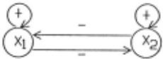
A qualitative model shown in Fig. 4b has an invari­ ant sign pattern x, = ( +-) and hence (- +) (If a qualitative model has a. invariant sign pattern x., then -x, also.) For example, (x,)! = +is preserved for all the time, since feed back circuit from both x 1 itself and x2 keep x1 increasing. Similarly, sign patterns of ( x s )2 are also preserved. Thus, the subpattern ( + 0) and (0 -) will fall into the sign pattern ( + -) by theorem 3.13. Further, it is also known by theorem 3.15 that this model has an equilibrium point in subspace ( + +) or (--)in case the system has a constant mode.

As we have known that the qualitative model of the pressure regulator example is potentially stable, it does not have any invariant sign pattern. The model does not have a non-zero equilibrium point.

4 Conclusion

We have shown that such global properties as stability and observability can be investigated purely from the qualitative information of dynamical interaction.

So far we have discussed a global analysis of a linear system. As often done in system theory, the results of linear system can be used for non-linear systems in the following three manners:

1. Non-linear systems can be approximated as linear systems in the neighborhood of the equilibrium point as in the example 2.1, and hence the results for linear systems hold there.
2. The results of linear system dxjdt =Ax holds for the non-linear system dxjdt = A(t)x if the change of A(t) is very slow.
3. By locally invariant heuristics, some properties such as stability of the system dxjdt =Ax+ f · F(x, t) do not ch~nge from that of dxjdt =Ax iff is sufficiently small.

We can use these approaches to the qualitative anal­ ysis for the non-linear system. That is, we divide the non-linear system into a set of linear systems each of which is an approximation of the non-linear system at some point and the neighborhood of the point. Sum­ ming up the results of these linear systems, the qual­ itative aspects of the non-linear systems are analyzed. Implementation of such an inference engine that syn­ thesizes the results of global properties of non-linear systems is left for future work.

can potentially exist is specified by solving the possible sign pat­ tern for 0 = f(x) .