
Discovering Admissible Models of Complex Systems Based on Scale-Types and Idemtity Constraints
Proceedings of the Fifteenth International Joint Conference on Artificial Intelligence. Learning. Pages 810-818.
© 1997 International Joint Conferences on Artificial Intelligence
Abstract
SDS is a discovery system from numeric measurement data. It outperforms the existing systems in every aspect of search efficiency, noise tolerancy, credibility of the resulting equations and complexity of the target system that it can handle. The power of SDS comes from the use of the scale-types of the measurement data and mathematical property of identity by which to constrain the admissible solutions. Its algorithm is described with a complex working example and the performance comparison with other systems are discussed.
- [Langley et al., 1985] P.W. Langley, H.A. Simon, G. Brad- shaw and J .M. Zytkow. Scientific Discovery; Computa- tional Explomtions of the Creative Process. MIT Press, Cambridge, Massachusetts, 1987.
- [Koehn and Zytkow, 1986] B. Koehn and J .M. Zytkow . Experimeting and theorizing in theory formation. Proceedings of the International Symposium on Method- ologies for Intelligent Systems, pages 296-307, 1986. ACM SIGART Press.
- [Falkenhainer and Michalski, 1985] B.C. Falkenhainer and R.S. Michalski. Integrating Quantitative and Quali- tative Discovery: The ABACUS System. In Machine Learning, pages 367-401, Boston, 1986. Kluwer Aca- demic Publishers.
- [Nordhausen and Langlay, 1990] B. Nordhausen and P.W. Langlay. An Integrated Approach to Empirical Discov- ery. Computational Models of Scientific Discovery and Theory Formation. Morgan Kaufman Publishers, Inc, San Mateo, California, 1990.
- [Wu and Wang, 1989] Y. Wu and S. Wang. Discovering Knowledge from Observational Data. In: Piatetsky- Shapiro, G. ed. Knowledge Discovery in Database, IJCAI-89 Workshop Proceedings, pages 369-377, 1989.
- [Schaffer, 1990] C. Schaffer. A Proven Domain-Independent Scientific Function-Finding Algorithm. Proceedings Eighth National Conference on Artificial Intelligence, pages 828-833, 1990. AAAI Press/The MIT Press.
- [Huang and Zytkow, 1996] K.M. Huang and J .M. Zytkow. Robotic discovery: the dilemmas of empirical equations. [Kokar, 1985]
- M.M. Kokar. Determining Arguments of In- variant Functional Descriptions. In Machine Learning, pages 403-422, Boston, 1986. Kluwer Academic Pul:>- lishers.
- [Buckingham, 1914] E. Buckingham. On physically similar systems; Illustrations of the use of dimensional equa- tions. In Physical Review, Vol.IV, No.4, pages 345-376, 1914.
- [Ljung, 1987] L. Ljung. In System Identification Theory for the User, 1987. PTR Prentice Hall, Englewood Cliffs, New Jersey.
- [Stevens, 1946] S.S. Stevens. On the Theory of Scales of Mea- surement. In Science, pages 677-680, 1946.
- [Bridgman, 1922] P.W. Bridgman. In Dimensional Analysis, 1922. Yale University Press, New Haven, CT.
- [Kanet al., 1972] M. Kan., N. Miyata and K. Watanabe. Research on Spaciousness. In Japanese Journal of Ar- chitechture, No.193, pages 51-57, 1972.
- [Washio and Motoda, 1997] T. Washio and H. Motoda. Discovery of First Principle Based on Data-Driven Rea- soning. Proc. of the First Pacific-Asia Conference on Knowledge Discovery and Data Mining, pages 169-182, 1997. Singapore.
- [Bshouty, 1994] D. Bshouty and N.H. Bshouty. On Learning Arithmetic Read-Once Formulas with exponentiation. Proc. of the Seventh Annual ACM Conference on Com- putational Learning Theory, pages 311-317, 1994. New Brunswick, NJ.
References were extracted automatically from the PDF and may contain errors.
Full text extracted automatically from the PDF; figures, tables and equations may differ. The PDF is the version of record.
1 Introduction
Finding regularities in the data is a basis of knowledge :u:quisitio? ~y ind.uction. One such typical and challeng mg task IS mducmg quantitative formulae of scientific laws from measurement data. Langley and others' BA CON systems [Langley et al., 1985] are most well known as the pioneering work. They founded the succeeding BACON family. FAHRENHEIT [Koehn and Zytkow, 1986], ABACUS [Falkenhainer and Michalski, 1985], IDS [Nordhausen and Langlay, 1990] and KEPLER [Wu and Wang, 1989] are such successors that basically use simi l~ algorith'?s to BACON in search for a complete equa twn govermng the data measured in a continuous pro cess. However, recent work reports that there is con siderable ambiguity in their results under noisy data even for the relations among small number of quanti ties [Schaffer, 1990; Huang and Zytkow, 1996]. Another drawback of the BACON family is the complexity of hy pothesis generation. This also limits their applicability to find a complex relation that holds among many quan tities.
To alleviate these drawbacks, some members of the BACON family, e.g. ABACUS, utilizes the informa tion of the quantity dimension to prune the meaningless ~erms based on the principle of dimensional homogene Ity. However, this heuristic still leaves many types of equations in candidates. COPER [Kokar, 1985], another t~e of. equation finding systems based on a principle of dimenswnal analysis called "Buckingham's IT-theorem"
[Buckingham, 1914], can significantly reduce the candi date generation by explicit use of the information about the quantity dimension. Its another significant advan tage is higher credibility of the solution that it is not merely an experimental equation but is indeed a first principle equation. However, these approaches are not applicable when the information of the quantity dimen sion is not available. This fact strongly limits their ap plicability to non-physics domains.
The primary objective of this study is to establish a me~hod to discover an admissible complete equation gov ermng a complex system where its domain is not lim ited to physics ensuring as much as possible its prop erty being the first principles. Any other technical ar eas, including system identification theory [Ljung, 1987], have not addressed to automatically derive first princi ple based models of complex systems from measurement data. Our goal if attained will provide an advantageous means not only for the field of scientific discovery but also for the analysis of complex systems in engineering. ~s a step towards this goal, we developed a quantita tive model discovery system "Smart Discovery System (SDS)" implementing our new approach. SDS utilizes newly introduced constraints of scale-type and identity both of which highly constrain the generation of candi date terms. Because these are not heuristics but mathe mati.cal constraints, the generated candidates are highly credible. SDS also adopts bi-variate equation generation based on data fitting. But what makes SDS different from BACON family is that it employs triplet checking of the validity of those bi-variate equations, a quite str~ng mathematical constraint. It should be emphasized that SDS does not require the information about quantity dimension. The information required besides the mea surements is the knowledge of scale-type of each quan t~ty. This feature expands the scope of its applicability smce the knowledge of scale-types is widely obtained in various domains including psychophysics, sociology and etc.
2 Outline of Method
SDS requires two assumptions on the feature of the ob jective system to be analyzed. One is that the objective system can be represented by a single quantitative, continuous and complete equation for the quantity ranges of our interest. Another is that all of the quantities in the equation can be measured, and all of the quantities except one dependent quantity can be controlled to their arbitrary values in the range. The latter is a common assumption in BACON family. The former is the as sumption of the original BACON systems, and is also assumed by other BACON family (i.e., search made for a complete equation for every continuous region in the objective system).
The information required from the user besides the actual measurements is a list of the quantities and their scale-types. The rigorous definition of scale-type was given by Stevens[Stevens, 1946]. He defined the mea surement process as "the assignment of numerals to ob ject or events according to some rules." He claimed that different kinds of scales and different kinds of measure ment are derived if numerals can be assigned under dif ferent rules, and categorized the quantity scales based on the operation rule of the assignment. The quantitative scale-types are interval scale, ratio scale and absolute scale, and these are the majorities of the quantities. Ex amples of the interval scale quantities are temperature in Celsius and sound tone where the origins of their scales are not absolute, and are changeable by human's defi nitions. Its operation rule is "determination of equality of intervals or differences', and its admissible unit con version follows "Generic linear group: x' = kx + c". Examples of the ratio scale quantities are physical mass and absolute temperature where each has an absolute zero point. Its operation rule is "determination of equal ity of ratios', and its admissible unit conversion follows "Similarity group: x' = kx". Examples of the absolute scale quantities are dimensionless quantities. It follows the rule of "determination of equality of absolute value', and "Identity group: x' = x" . Here, we should note that the scale-type is different from the dimension. For in stance, we do not know what the force (ratio) divided by the acceleration (ratio) means within the knowledge of scale-types.
In the following sections, the details of the algorithm of SDS are explained. For clarification purpose, we first focus on the case where the model involves only ratio and absolute scales in the next section. The extension to interval scale is described in the latter section. SDS can handle all of the three scale-types.
3 Equation Search Based on Ratio Scale
3.1 Bi-Variate Test
The algorithm of SDS is outlined in Figure 1. Step (1-1) significantly reduces the search space of bi-variate equa tions by using the "scale-type constraint." Two well known theorems in the dimensional analysis provides the basis of this step [Buckingham, 1914].
Buckingham IT-theorem If ¢(x, y, .... ) = 0 is a com plete equation, and if all of its arguments are either ratio or absolute scale-types, then the solution can be written Given a set of ratio scale quantities, RQ, and a set of absolute scale quantities, AQ,
- {1-1) Apply bi-variate test for an admissible equa tion of ratio scale to every pair of quantities in RQ. Store the resultant bi-variate equa tions accepted by the tests into an equation set RE and the others not accepted into an equation set N RE.
- {1-2) Apply triplet test to every triplet of associ ated bi-variate equations in RE. Derive all maximal convex sets for the accepted triplets, and compose all bi-variate equations into a multi-variate equation in each maximal con vex set. Define each multi-variate equation as a term. Replace the merged quantities by the generated terms in RQ.
- {2) Let AQ = AQ + RQ. Given candidate for mulae set CE, repeat steps {2-1) and {2-2) until no more new term become generated.
- {2-1) Apply bi-variate test of a formula in CE to every pair of the terms in AQ, and store them to AE. Merge every group of terms into a unique term respectively based on the result of the bi-variate test, if this is possible. Replace the merged terms with the generated terms of multi variate equations in AQ.
- {2-2) Apply identity constraints test to every bi-variate equation in AE. Merge every group of terms into a unique term re spectively based on the result of the iden tity constraints test, if they are possible. Replace the merged terms with the gen erated terms of multi-variate equations in AQ. Go back to step {2-1) .
The candidate models of the objective system are derived by composing the terms in AQ.
Figure 1: Outline of SDS algorithm
in the form
where n is the number of arguments of¢, and r is the basic number of bases in x, y, z..... For all i, IIi is an absolute scale- type quantity.
Bases are such basic scaling quantities independent of the other bases in the given ¢, for instance, as length [L], mass [M] and time [T] of physical dimension. The relation of each IIi to the arguments of¢ is given by the following theorem [Bridgman, 1922].
Product Theorem Assuming primary quantities, x, y, z, ... are ratio scale-type, the function p relating a secondary quantity II to x, y, z, ... has the form:
where r, a, (3, 'Y, ... are constants.
These theorems state that any meaningful complete equation consisting only of the arguments of ratio and absolute scale-types can be decomposed into an equa tion of absolute scale-type quantities having an arbitrary form and equations of ratio scale-type quantities having products form. The former F(TI1, TI2, ... , lln-r) = 0 is called an "ensemble" and the latter n = p(x, y, z, ... ) = rx<>yf3 z"t ... "regime's.
Because we know that any pair of ratio scale quanti ties in a given complete equation has a product relation if both belong to an identical regime, SDS searches bi variate relations having the following product form in RQ, which is the unique admissible equation that hold in such a regime.
The value of the constant a must be independent of any other quantities according to Product Theorem, while the constant b is dependent on the other quantities in the regime. SDS applies the least square fitting of Eq. 1 to the bi-variate experimental data of x and y that are measured while holding the other quantities constant, and determines the values of a, its expected standard error da, and b. For ease of linear fitting, the logarithmic form ofEq.1, alogx+logy = Iogb, is used instead ofEq. 1 itself. The judgment is made whether this equation fits the data well enough by the following two types of statistical tests.
- F-test of the ratio between variances of regressive component SR = (CJx/ /CJyy) 2 and residual error component Se = CJ ee 2 ,
- test if da is larger than the absolute value of a itself.
The test (1) is to check if the equation accurately fits to the given data in terms of the power (variance) of residual component. The test (2) is to simply check if the value of the constant a is meaningful. When any of the tests fail, x and y are judged not to have the prod uct relation. For identical pair of ratio scale quantities, this procedure is repeated k = 10 times to check the independence of the constant a while holding the other quantities at randomly chosen different values. Then the following test is applied to the set of values of a and da to check the independence.
- x 2 -test of the ratio between variance of the values of a and the average of da over the k data set.
If all these tests are passed, the pair of x and y is judged to have the admissible product relation. Then the bi-variate equation together with the average of a and da, i.e., a and da is stored to RE. If any of the tests failed, the bi-variate equation, a and da are stored to NRE.
The procedure in step (1-1) is now demonstrated by an example of a complex system depicted in Figure 2. This is a circuit of photo-meter to measure the rate of increase of photo intensity within a certain time period. The resistance and switch parallel to the capacitor and the current meter are to reset the operation of this cir cuit. The actual model of this system is represented by the following complex equation involving 17 quanti ties.
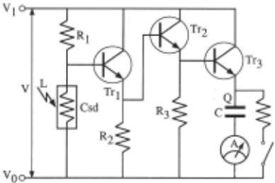
Here, L and r are photo intensity and sensitivity of the Csd device. X, K and Bare position of indicator, spring constant and intensity of magnetic field of the current meter respectively. hie; is input impedance of the base of the i-th transistor. hte; is gain ratio of the currents at the base and the collector of the i-th transistor. The definitions of the other quantities follow the standard symbolic representations of electric circuit (See Figure 2). Only hfe;S are absolute scale, and the rest are ratio scale. X is the dependent quantity in this circuit, and the others are independently controllable by the change of boundary conditions and the replacement of devices. SDS requests the bi-variate change of quantities to the experimental environment. When it is told that a quan tity is dependent (not controllable) during the search process, SDS modifies its request to control the other independent quantity. A simulation based experimental environment was prepared for the circuit system. ±4% (std.) of relative Gaussian noise was added to both of the control quantity (input) and the measured quant ity (output) in every bi-variate test. First, SDS set RQ as {V, L, r, R1, R2, R3, hiep hie 2 , hie~, Q, C, X, K, B} and AQ as {hteu ht<:.·· hte~} based on the input information on scale-types. l~ext, 1t performed the bi-variate fitting of a product form among the quantities in RQ, and ap plied the statistical tests of (1)-(3) . The following shows the values of F for F -test, the power constant a and its std. errors da resulted in the bi-variate test for x = Q and y = X under k = 10 combinations of different values of the other quantities.
| 1: | F=25.93 | a= | 0.6682 da=0.0100 |
| 2: | F=1.986 | a= 0.6339 | da=0.0346 |
| 3: | F=0.748 | a= 0.4840 | da=0.1086 |
| 4: | F=27.08 a= | 0.6789 | da=0.0100 |
| 5: | F=1.421 a= | 0.5833 | da=0.0640 |
| 6: | F=0.405 a= | 0.3902 | da=0.1539 |
| 7: | F=0.860 a= | 0. 2351 | da=0.6268 |
| 8: | F=37.09 | a= 0.7655 | da=0.0100 |
| 9: | F=1.843 | a= 0.6226 | da=0.0424 |
| 10: | F=6.324 | a=-0.0494 | da=0.0557 |
IfF < 5.317 then the test (1) fails, and if da > lal then the test (2) fails. Many iterations failed either one of the tests (1) and (2). For the test (3), x 2 = 39.54 was obtained where it was larger than the threshold value 16.92. Thus, this test also failed. The resultant RE of the bi-variate equations that were passed the tests was as follows.
All pairwise product forms that should hold among the quantities in RQ have been correctly enumerated.
3.2 Triplet Test
In the next step (1 - 2), triplet consistency tests are applied to every triplet of equations in RE. Given a triplet of the power form equations in RE:
by substituting yin the first toy in the second, we obtain
Thus, the following condition must be met.
However, if any of the three equations are not correct due to the noise and error of data fitting, this relation may not hold. The following test judges if the three of the equations are mutually consistent in terms of as.
- Given Erra = axz + ayzaxy and its expectation -2 - - 2 - - 2 1/2 EXPda = { daxz + ( dayzaxy) + ( ayzdaxy) } , perform normal distribution-test of Erra based on its expectation Expda·
SDS applies this test to every triplet of equations in RE, and search every maximal convex set M C S where each triplet of equations among the quantities in this set has passed the test (4). In addition, every pair of quanti ties in an equation in RE which does not belong to any triplet such as Eq.3 is also regarded as a tiny MCS, because the equation may be a regime. When actual regimes in the objective system are mutually indepen dent, each MCS will correspond to a regime. However, an MCS may be different from the set of quantities in a real regime stated in Buckingham IT-theorem in the following cases.
- (A) Product of two regimes in an ensemble If two real regimes II1 = x1a"' 1 y1av 1 ··· and II2 = x 2a"' 2 y2av 2 ··· have a relation of product in their en semble as F(II1 an1 II2an2 , ··· , IIn-r) = 0, then MCS will be a superset of the quantities of the two real regimes.
- (B) Common terms between two regimes If two real regimes II 1 = X1 axl Y1 a11 1 ··· sa·1 rat1 ... and II2 = x2ax 2 y2av 2 ··· Sa· 2 Ta' 2 ··· share some common terms S, T, ... , then the partition of the set of quan tities in each regime {x1, Y1, ... }, {x2, Y2 · ... },{PIPE S}, {qlq E T}, ... will become MCSs.
In case of (B), sa· 1 Tat1 and sa· 2 Ta' 2 can be rq and pq 2 respectively for instance, where S = p and T = q. Then {p} and {q} are MCSs. In another case, if S = P1P2P3 and T = q1q2 2 , then {P1,P2,P3} and {q1,q2} are MCSs. These facts also hold for more than two regimes. These consideration indicates that every MCS does not have any intersection with others in any case. If any MCSs mutually sharing some quantities are obtained, those MCSs may not be valid due to the noise and error of the data fitting in step (1-1). It means some pairwise product forms among the elements of those M C Ss have been missed in the tests. Accordingly, the following test and operation are applied to the resulted MCSs.
- Given a set of MCSs S = {M1 ,M2 , ··· } where each Mi shares some quantities with the other el ements inS, obtain the merged MCSs,i.e., Ms = uM,ESMi, if p ::; Pth. by assuming that the Mis in S have been obtained because of missing p pairwise product forms among the elements in Ms. Then move the p pairwise product forms from N RE to RE.
The valid number pis always given by the following ex pression.
where f(M) = IM I (I~I - 1 ) is the number of the pairwise links in a set M, 2 8 is the power set of S, and IAI is the cardinality of A. Pth is empirically set to be 3 in SDS. The calculation of Eq.5 is limited to lSI ::; 3, because p always exceeds 3 for lSI > 3. For example, when S = { { x1, x2, Y1 }, { x1, x2, Y2}, { x1, x2, y3}} has been derived, we once assume M8 = {x1, x2, Y1, y2, Y3}· The number of missing pairwise product forms is calculated as
where p is equal to Pth· Thus, three pairs of quantities in Ms, {y1, Y2}, {y2, Y3} and {y3, Y1}, which do not be long to any of {x1,x2,Y1}, {x1,x2,Y2} and {x1,x2,y3}, are moved from NRE toRE. Once all MCSs are found, the data-driven regimes are given by the following form.
ais and their std. errors dais are evaluated by the aver age of a and da of the equations in RE. Before the final value of ai is determined, the following test is applied.
- normal distribution-test to check if ai is close to an integer under the error dai. If ai is judged to be an integer, it is set to the integer value.
This test is based on the observation that the majority of the first principle based equations have integer power coefficients. The product form given by Eq.6 is named as a pseudo-regime to distinguish it from the real regime. As we see, the ITs given by pseudo-regimes are not guar anteed to be dimensionless (absolute scale), and also the pseudo-regimes do not share any quantities mutually, even when the original regimes share some quantities. Finally, the merged quantities are replaced by the term of each equation of the derived pseudo-regime in RQ.
In the example in Figure 2, after performing the triplet test of (4) for theRE, the resultant MCSs did not mu tually share any quantities, and thus, they are combined in the form of Eq.6 skipping the test (5). Subsequently, their power coefficients were evaluated by the test (6), and they were known to be integer values. The final forms of pseudo-regimes replaced the merged terms in RQ in this step as follows.
4 Searching Ensemble Equations
4.1 Generation of Terms based on Bi-Variate Test
Once all pseudo-regimes are identified, new terms are generated in step (2-1) by merging these pseudo-regimes in preparation to compose the ensemble equation. First, RQ is added to AQ. Subsequently, SDS searches bi variate relations having one of the formulae specified in the equation set CE. The repertoire in CE governs the ability of the equation formulae search in SDS. Cur rently, only the following two simple formulae are given in CE. Nevertheless, SDS performs very well in search for the ensemble equation.
First, SDS adopts the least square fitting of Eq. 7 as in step(1-1). Then, the statistical tests (1) and (2) mentioned earlier are applied. This process is repeated k = 10 times for randomly chosen different combinations of the values for the other quantities in AQ. If all these tests are passed, the bi-variate equation is stored to AE, and the test (3) is conducted to check the independence of a. Note that this test is not used to reject the relation here because x and y may be absolute scale, and thus a can depend on the other quantities in AQ. SDS marks the relation having the independent a in AE. After all pairwise relations in AQ are examined, SDS searches ev ery maximal convex set MCS as in step(1-2) for the relations marked as the independent a, and the quanti ties in an M C S are merged into the following term.
Similar procedure is applied to Eq.8, in which case the merged term of an MCS is:
This procedure is repeated in couple for both Eqs. 7 and 8 until no new term becomes possible. If all terms in AQ is merged into one, the equation of the final term is the ensemble equation.
In the example of the circuit, Eq.7 was applied first , and three MCSs were found. They were merged to the following new terms.
Next, Eq.8 was tested, then one MCS was found.
AQ became as {81, 82, 83, 84, II6, }. Again, by apply ing Eq.7, another MSC was newly generated.
Thus, AQ = {81, 82, 83, 8s}. As no new terms became available, this step was finished.
4.2 Generation of Terms based on Identity Constraints
In step (2-2), the identity constraints are applied for fur ther merging terms. The basic principle of the iden tity constraints comes by answering the question that "what is the relation among 8h, 8i and ej, if 8i = fej (8h) and 8i = fe, (8h) are known?" For example, if a(8j)8h + 8i = b(8j) and a(8i)8h + 8j = b(8i) are given, the following identity equation is obtained by solving each for 8h.
Because the third expression is linear with 8i for any 8i, the second must be so. Accordingly, the following must hold.
By substituting these to the second expression,
is obtained. This principle is generalized to various re lations among multiple terms. Table 1 shows such rela tions for multiple linear relations and multiple product relations. SDS checks every bi-variate equation in AE derived in step (2-1). If a bi-variate linear equation has a that depends on other terms, it is stored in a set L, and if a bi-variate product relation has such a, it is stored in P. Then the bi-variate least square fitting of the general relations indicated in Table 1 is applied to AQ. For ev ery bi-variate fitting and their coefficients, the test (1) , (2) and (3) are also conducted. If all the coefficients ex cept one are independent in a relation, the relation is solved for the unique dependent coefficient, and the co efficient is set to be the merged term of the relation. If all coefficients are independent in a relation, the relation is the ensemble equation. If such ensemble equation is not found, SDS goes back to the step (2-1) for further search.
| bi-variate relation | general relation |
|---|
L is a set of pairwise terms having a bi-variate linear relation and LQ = UpELP· P is a set of pairwise terms having a bi-variate product relation and PQ = UpEPP·
In the example of the circuit, SDS found a set of the bi-variate linear relations in AE. These were on the combinations of {81, 8 5}, {82, 8 5} and {83, 8 5}. By applying the bi-variate fitting of the general linear equa tion in Table 1, the following multi-linear formula has been obtained.
Because every coefficient is independent of any terms, this is considered to be the ensemble equation. The equivalence of this result to Eq.2 is easily checked by sub stituting the intermediate terms to this ensemble equa tion.
5 Equation Search Based on Interval Scale
The conventional Buckingham II-theorem and Product Theorem do not consider the equation involving interval scale quantities. We have extended these theorems to include interval scales[Washio and Motoda, 1997].
Extended Buckingham II-theorem If ¢(x1 , x2 , x3 .... ) = 0 is a complete equation, and if each argument is one of interval, ratio and absolute scale-types, then the solution can be written in the form
where n is the number of arguments of¢>, w is the basic number of bases in x 1,x2 ,x3 ·.·· , respectively. For all i, IIi is an absolute scale-type quantity.
Extended Product Theorem Assuming primary quantities in a set R are ratio scale-type, and those in another set I are interval scale-type, the function p relat ing a secondary quantity II to xi E R U I has the forms:
where all coefficients except II are constants and hni 9 = ¢.
These theorems state that any meaningful complete equation consisting of the arguments of interval, ratio and absolute scale-types can be decomposed into an en semble having an arbitrary form and regimes of inter val and ratio scale-type quantities in products and log arithmic form. In each regime, every interval scale-type quantities appears in linear relation with some other in terval scale-type quantities. Therefore, specific tasks in the equation search associated with interval scale quan tities are to seek linear forms among interval scale-type quantities and to seek the logarithmic relation between a linear form and the others. For these tasks, the steps in dicated in Figure 3 are inserted in the original algorithm of SDS.
Additionally given a set of interval scale quanti ties, IQ,
- (0-1} Apply bi-variate test for an admissible lin ear equation of interval scale to every pair of quantities in IQ. Store the resultant bi variate equations accepted by the tests into an equation set IE and the others not ac cepted into an equation set N IE.
- (0-2} Apply triplet test to every triplet of associ ated bi-variate equations in IE. Derive all maximal convex sets MCSs for the accepted triplets, and compose all bi-variate equations into a multi-variate equation in each MCS. Define each multi-variate equation as a term. Replace the merged terms by the generated terms of the multi-variate equations in IQ. Let RQ = RQ + I Q.
- (1-3} Apply bi-variate test for an admissible loga rithmic equation between the linear forms of interval scale-type quantities and the other terms in RQ. Replace the terms in the re sultant bi-variate equations accepted in the tests by the generated terms in RQ.
Figure 3: Extended part of algorithm
The step (0-1) and (0-2) are almost identical with the steps (1-1) and (1-2) except that the foilowing admissible relation is used at the bi-variate data fitting in IQ.
Once a multi-variate linear form is obtained after the triplet test, the form is dealt with a term in the regime formulae based on the extended Product Theorem, and the te.rm is stored into RQ by IQ. In step (1-3), the followmg bi-variate logarithmic relations are sought be tween the linear forms of interval scale-type y and the other terms x in RQ.
!he triple~ test is not applied at this step because Eq.12 lS asymetnc and essentially a bi-variate relation.
In case of the aforementioned example, the circuit does not involve any interval scale-type quantities. However, if we look the electric voltage not to be a voltage differ ~nce V but two voltage levels V0 and V1 , they become mterval scale-type. Hence, the system is represented by the following 18 quantities.
IQ {Vo, Vl},
AQ = {hfep hfe2' h/e3}.
SDS applied the step(O) to the experimental data, and figured out a term 8o = V1 - V0 quickly. The rest of the reasoning was identical with the description in the previous sections.
6 Discussion and Related Work
Main features of the discovery system SDS are its low complexity, robustness, scalability and wide applicabil ity. The basic algorithm of SDS consists of two types of procedures. One is the bi-variate test for each pair of quantities and terms in steps (0-1), (1-1), (1-3) and (2-1). The complexity of this type of procedure is O(n 2 .m 2 k) where n, m, k are the number of quantities to represent the objective system, the number of experimental data used for a data fitting and the number of iteration of the data fitting in a bi-variate test, respectively. Another is the triplet test for each triplet of quantities and terms in steps (0-2), (1-2) and (2-2), where its complexity is O(n 3 ). m and k usually do not affect the performance of SDS as they are almost independent of the complexity o.f objective system structure. Moreover, the computa tiOnal cost required in the bi-variate test is much larger than the triplet test because the former involves multi ple ~xperiments, data sampling, data fitting and some stat1st1cal tests, whereas the latter involves the triplet consistency checking among the given coefficients only. Thus, the practical complexity is almost proportional to the second order of n. Table 2 shows the performance of SDS to discover various physical law equations. The relative CPU time of SDS normalized by the first case shows that its complexity is nearly proportional to n 2 . For reference, the relative CPU time of ABACUS is indi cated for the same cases except for the circuit examples of this paper[Falkenhainer and Michalski, 1985]. Though ABACUS applies various heuristics including the infor mation of dimension, its complexity is still NP-hard. As thi~ feature is shared by BACON family, they can hardly denve the model of the electric circuit of this complexity.
The robustness of SDS against the noisy experimental environment has been also evaluated. The upper limita tion of the noise level to obtain the correct result in the cases of more than 80% of 10 trials was investigated for each physical law, and they are indicated in the last col umn of Table 2. The noise levels shown here are the std. of Gaussian noise relative to the real values of quantities, and were added to both controlled (input) quantities and measured (output) quantities at the same time. Thus ac tual noise level is higher than these levels. The results show the significant robustness of SDS. SDS can provide appropriate results under any practical noise condition.
| Example | n | TC(S) | TC(A) | NL(S) |
|---|---|---|---|---|
| Ideal Gas | 4 | 1.00 | 1.00 | ±40% |
| Momentum | 8 | 6.14 | 22.7 | ±35% |
| Coulomb | 5 | 1.63 | 24.7 | ±35% |
| Stoke's | 5 | 1.59 | 16.3 | ±35% |
| Kinetic Energy | 8 | 6.19 | 285. | ±30% |
| Circuit*! | 17 | 21.6 | ±20% | |
| Circuit*2 | 18 | 21.9 | ±20% |
The low complexity and the high robustness shown ?ere ensure the significant scalability of SDS to engineer mg problems. Many systems in BACON family adopt generate and test in the search. In contrast the low c?mplexity of SDS comes from its straightforV.:ard algo nthm to apply only product and linear forms in polyno mial time order in concert with the highly restrict ive but domain independent constraints. By adding some more basic functional equations to CE, the search of SDS will become more powerful. The robustness of SDS comes from the bi-variate direct fitting to data and the struc ture of the triplet test. The systems in BACON family repeat formulae fitting to coefficients resulted from the other fitting if it is necessary. This method accumulates the error of data fitting, and derives erroneous results. On the other hand, SDS uses only the bi-variate and di rect fitting to the given data, and efficiently composes the result in statistically accurate manner. The multi ple statistical tests provide quite conservative judgment on the selection of equations, which contributes to re ducing the ambiguity of reasoning. But it also requires following up of missed equations. This is done by re constructing M C Ss in the triplet test by assuming some missed equations in the derived MCS.
~he wide applicability is another advantage of SDS, as 1t does not require any information on dimensions of quantities. For example, the following equation is known to be the law of spaciousness of a room in psychophysics[Kanet al., 1972].
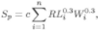
where Sp, R, Li and Wi are average spaciousness of a room, room capacity, average light intensity and solid angle of window at the location i in the room. Though the dimension of Sp is unclear, its scale-type is known to be ratio scale based on its definition. L and R are ratio scale, and W is absolute scale. We applied SDS to this system for the case of n = 3, and easily obtained the above expression. The dimension based approach such as COPER may not be applicable to this case.
The weakness of the approach of SDS is some lim its on the class of formulae to be discovered. First, the regimes and ensemble formulae must be read-once formulae, where each quantity appears at most once in it. Second, the relations among quantities must be arithmetic, where the operators are limited to addition, subtraction, multiplication, division, exponentiation and logarithm because of the limited contents of CE. Third, the formula of every pair of quantities searched in the bivariate test is limited to the relation of a simple bi nary operator. These restrictions should be relaxed, even though the majorities of the first principle for mulae fall into this class. Bshouty et al. proposed an approach to find three unary arithmetic functions g(x), h(y) and /(·) related by a binary arithmetic op erator, e.g., f(g(x) + h(y)) for a given arithmetic rela tion F(x, y). It is based on an invariance principle of this structure under the linear conversion of g(x) and h(y)[Bshouty, 1994]. Their approach may not be very adequate for the data-driven discovery, because it as sumes an initially given precise relation of F(x, y) and its derivatives. However, this invariance principle on the binary relation has a possibility to provide an efficient remedy to the third limi tation. The second limitation can be relaxed by increasing the variety of the contents of CE. The first is also a challenging issue, and some invariance or identity principle can be used for the re laxation. All of these issues are left for the future work.
7 Conclusion
SDS implements newly introduced constraints of scale type and identity in the algorithm of bi-variate and triplet equation test. This architecture has shown to have low complexity, high robustness, promising scala bility and wide applicability. It is true that the most of the scientific discoveries have been made through a large number of experiments and observations. However, the scientists have not solely relied on the data but some admissible conditions such as invariance of light speed, symmetry for time inverse and continuity of relations. The constraints of scale-type and identity are two of such conditions having wide applicability. Our future plan is to extend this work to further larger systems and also to seek new laws in non-physical domains.
@inproceedings{ijcai1997p117,
  title     = {Discovering Admissible Models of Complex Systems Based on Scale-Types and Idemtity Constraints},
  author    = {Washio, Takashi and Motoda, Hiroshi},
  booktitle = {Proceedings of the Fifteenth International Joint Conference on
               Artificial Intelligence, {IJCAI-97}},
  publisher = {International Joint Conferences on Artificial Intelligence},
  editor    = {Martha E. Pollack},
  pages     = {810--818},
  year      = {1997},
  note      = {Learning},
  url       = {https://ijcai.org/proceedings/1997/117},
}
TY - CPAPER TI - Discovering Admissible Models of Complex Systems Based on Scale-Types and Idemtity Constraints AU - Washio, Takashi AU - Motoda, Hiroshi T2 - Proceedings of the Fifteenth International Joint Conference on Artificial Intelligence, IJCAI-97 PB - International Joint Conferences on Artificial Intelligence PY - 1997 SP - 810 EP - 818 UR - https://ijcai.org/proceedings/1997/117 ER -Copied
Machine-readable versions of this paper, for tools and AI agents:





