
Extracting Constraint Satisfaction Subproblems
Proceedings of the Fourteenth International Joint Conference on Artificial Intelligence. Constraint Satisfaction. Pages 548-556.
© 1995 International Joint Conferences on Artificial Intelligence
Abstract
Given a subproblem, S, of a constraint satisfaction problem, we can decompose the problem into a set of disjoint subproblems one of which will be S. This decomposition permits exploitation of problem-specific metaknowledge, a priori or acquired knowledge, about S. If we know that S is unsolvable, for example, the decomposition permits us to extract and then discard S, restricting the search for a solution to the remaining subproblems. A variety of potential uses for the decomposition method are discussed. A specific method that dynamically discards failed subproblems during forward checking search is described, and its utility demonstrated experimentally.
- Charman, P., Solving space planning problems using constraint technology, in Nato ASI Con- straint Programming: Students' Presentations, TR CS 57/93, Institute of Cybernetics, Estonian Academy of Sciences, Tallinn, Estonia, 80-96.
- Cheeseman et al. 91]
- Cheeseman, P., Kanefsky, B. and Taylor, W., Where the really hard problems are, IJCAI-91, 331-337. IJCAI
- Freuder, E . Complexity of k-tree struc- tured constraint satisfaction problems, AAAI-90, 4-9.
- Freuder and Hubbe 93]
- Freuder, E. and Hubbe, P., Using inferred disjunctive constraints to decompose con- straint satisfaction problems, IJCAI-93, 254-261. IJCAI
- Freuder and Hubbe to appear] Freuder, E. and Hubbe, P., A disjunctive decomposition control schema for constraint satisfaction, in Principles and Practice of Constraint Programming, V.J. Saraswat and P. Van Hen- tenryck, eds., The MIT Press.
- Frost and Dechter 94] Frost, D. and Dechter, R., Dead-end driven learning, AAAI-94, 294-300.
- Haralick and Elliott 80]
- Haralick R. and Elliott, G. , Increasing tree search efficiency for constraint satisfac- tion problems, AIJ 14, 263-313. IJCAI
- Hubbe and Freuder 92] Freuder, E. and Hubbe, P., An efficient cross product representation of the constraint satisfaction problem search space, AAAI-92, 421-427.
- Mackworth, A. , On reading sketch maps, IJCAI-77, 598-606.
- Nadel, B., Constraint satisfaction algo- rithms, Computational Intelligence 5, 188-224.
- Prosser, P., Hybrid algorithms for the con- straint satisfaction problem, Computational Intelligence 9, 268-299.
- Sabin and Freuder 94]
- Sabin, D. and Freuder, E. , Contradicting conventional wisdom in constraint satis- faction, in Principles and Practice of Constraint Pro- gramming, LNCS 874, A. Borning, ed., Springer-Verlag, 10-20.
- Schiex and Verfaillie 93
- Schiex, T. and Verfaillie, G., Nogood recording for static and dynamic constraint sat- isfaction problems, TAl '93, 48-55.
- Smith and Kelleher 88]
- Smith, B. and Kelleher, G., Reason Maintenance Systems and Their Applications, Ellis Horwood, Chichester, England.
- Verfaillie
- Verfaillie, G. personal communication. [Williams and Hogg 92]
- Williams, C. and Hogg, T., Using deep structure to locate hard problems. AAAI- 92, 472-477.
- van Beek 94] van Beek, P., On the inherent level of local consisttency in constraint networks,AAAI-94, 368- 373.
- Hentenryck 89
- Van Hentenryck, P., Constraint Satisfaction in Logic Programming, MIT Press.
References were extracted automatically from the PDF and may contain errors.
Full text extracted automatically from the PDF; figures, tables and equations may differ. The PDF is the version of record.
1 Introduction
1.1 Overview
Constraint satisfaction problems ( CSPs) involve finding values for problem variables subject to restrictions (con straints) on what combinations of values are allowed. They have wide application in artificial intelligence, in areas ranging from planning to machine vision.
Fig. 1a shows a sample CSP. The problem is to assign a color to each vertex of the graph satisfying the restric tions that vertices joined by an edge cannot be assigned the same color. Coloring problems are useful for illus tration purposes (and actually have applications, e.g. to scheduling). They are in general NP-complete, though obviously the example here is a trivial one. The CSP variables in this coloring problem are the vertices of the graph. The domain of values for each variable is the set of colors available for the vertex; in this case colors a b c (aquamarine, black and coral) are available at each ~er~ tex. The constraints are the "not same color" (i.e. "not equal") restrictions corresponding to each edge. Call any choice of a value for each variable, e.g. a for X, b for Y, a for Z, a possibility. A possibility that satisfies all the constraints is a solution.
*This material is based on work supported by the National
Science Foundation under Grant No. IRI-9207633.
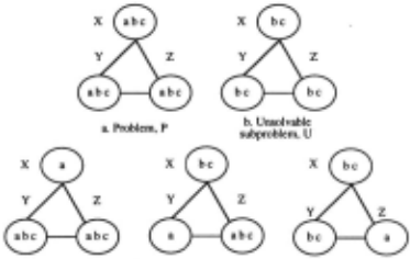
At times we may have special knowledge of a CSP subproblem and wish to extract it from the CSP, to de compose the CSP in a manner that permits us to con sider the subproblem and the remainder of the CSP sep arately. This paper provides a mechanism for doing so for a large class of subproblems.
For example, Fig 1b shows a subproblem of the col oring problem. This is an example of what we call here a subdomain subproblem, essentially one in which the domains of some variables have been reduced. This par ticular subproblem obviously has no solution. It repre sents a special case of the easily inferred conclusion that a complete graph of n vertices (one in which each pair of vertices is joined by an edge) cannot be colored with n-1 colors. The subproblem contains 8 of the 27 possibilities in the original problem, almost 30 per cent of the total. It would be nice if we could extract this subproblem, and then discard it. But what exactly would be left? Well, in fact, what is left are the three subproblems shown in Fig. 1c. One contains 9 possibilities, one 6, one 4. Together they contain precisely the 19 possibilities that remain when the subproblem in Fig. 1b is removed.
Our general extraction procedure provides a mech anism for exploiting many forms of "metaknowledge" about subproblems; it is described in Section 2. We use this scheme in a specific, new method that dynamically factors out, extracts and removes, failed subproblems, repeatedly during search; this is described in Section 3. Section 4 evaluates the new method experimentally on hard homogeneous and inhomogeneous problems. Sec tion 5 speculates on further uses for the general mecha nism; Section 6 is a brief conclusion.
1.2 Relation to Previous Work
The subproblem extraction method is a generalization of the IDC decomposition employed in [Freuder and Hub be 1993]. (Thus the IDC algorithm already provides one successful application of the extraction approach.) The IDC algorithm extracts and discard subproblems that may contain solutions, and thus is not appropriate when seeking all solutions (but is guaranteed not to discard all solutions). The basic decomposition step of the extrac tion method, dividing a problem into two subproblems, utilizes domain splitting [Mackworth 77; Van Henten ryck 89]; the extraction method combines several split ting operations for a specific new purpose.
Factoring out failed subproblems provides a new ap proach to profiting from experience during search, which we will imbed in a new algorithm called FOF for "fac tor out failure". There has, of course, been considerable work on learning or remembering new constraints dis covered during search in the CSP literature (e.g. [Frost and Dechter 94, Schiex and Verfaillie 93]) with connec tions to the truth maintenance literature, (see [Smith and Kelleher 88]). The closest to FOF is probably the learning method of Charman [Charman 93], but FOF has considerably more potential for pruning.
The failed subproblem could be recorded as a new k ary constraint. However, the overhead of remembering and employing such constraints is problematic. Initial experiments along this line did not demonstrate an im pressive performance, though this alternative approach may prove useful for problems with an appropriate struc ture [Verfaillie 93]. In fact, our approach is almost the opposite in spirit to traditional learning or TMS ap proaches. There individual "nogoods", inconsistent k tuples, are recorded and consulted for future pruning. With our approach entire subproblems are discarded, rather than remembered.
2 Extraction
For simplicity we restrict our attention here to binary CSPs, where the constraints involve two variables. A value for variable U and one for variable V are said to be consistent if they satisfy the constraint between U and V, i.e. the pair of values is permitted by the con straint. Tightness is a measure of how many pairs satisfy a constraint, the higher the tightness, the fewer consis tent pairs. Density is a measure of how often there is a constraint between pairs of variables, the higher the density, the more constraints there are.
The process that produced the decomposition of the example in the introduction is shown in Figure 2. The original problem appears at the root of the decompo sition tree. The decomposition consists of the leaves; since one of the subproblems is unsolvable here, it can be discarded. Problems are represented by the variable domains, where the variables are listed in lexicographic order.
We say that the decomposition extracts the target sub problem 8 from the original problem. The method can be generalized to extract any subdomain subproblem from any CSP. 8 is a subdomain subproblem of P if 8 can be obtained from P by eliminating some values from some of the variable domains (or in the trivial case, eliminating nothing). The extraction procedure:
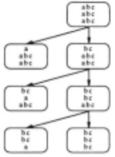
Extract (Subproblem, Problem, Decompositon) Until the Problem matches the target Subproblem Pick a variable, V, in the Problem whose domain does not match the target Subproblem Divide the Problem into two subproblems that differ only in that the domain of V in one matches the domain of V in the target Subproblem while the domain of V in the other contains the remaining values Set the Problem to the first of these subproblems; add the second to the Decomposition Apply Extract to the updated Problem and Decomposition with the same target Subproblem Return the Decomposition
If we invoke Extract initially with Decomposition Subproblem, it is easy to verify that the resulting de composition has the following properties:
- Each possibility for the original problem is con tained in one of the subproblems in the decomposi tion.
- Each subproblem possibility is a possibility for the original problem.
- No possibility is contained in more than one sub problem.
- The target subproblem is one of the subproblems.
Thus we have a disjoint, disjunctive decomposition of the original problem. Finding a solution for any one of the subproblems will solve the original problem. We measure the size of a problem simply by multiplying the number of values for each variable, to give the total num ber of possibilities. The size of the decomposition, mea sured as the sum of the sizes of the subproblems, is pre cisely the size of the original problem; the union of the possibilities of the subproblems is the set of possibilities for the original problem. If we wish to extract and dis card the target subproblem, we can invoke Extract with the empty set as the initial Decomposition.
3 Factoring Out Failure
3.1 Example
Subproblems without solutions may be discovered during search. We would like to be able to learn from that experience. We have developed an algorithm called FOF, factor out failure, which does this. We illustrate the idea with an elaboration, shown in Figure 3a, of the same simple problem we used in the Introduction. Assume the search order for variables and values is lexicographic order.
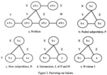
FOF is implemented as an extension of forward check ing [Haralick and Elliott 80], itself already one of the most successful algorithms in the literature. Forward checking is a variant of backtrack search. When a ten tative choice of a value for a variable is made forward checking removes from other variable domains all values inconsistent with the choice. If that leaves any domain empty, we have a failure. Failures can lead to backtrack ing. After choosing color a for variables U, V and W, forward checking is essentially left with a subproblem, Figure 3b, that is identical to the problem in Figure la. This, as we know, has no solution, and forward checking will eventually discover that, after trying various pos sibilities, and back up to choose another color, b, for variable W. At that point forward checking will face the new subproblem shown in Figure 3c.
The failed subproblem, F, and the new subproblem, N, have a lot in common, as we might expect, since the only changes were the ones incurred by the change of the choice of value for one variable. Figure 3d represents the intersection of the two subproblems, I; it contains those values, and thus those possibilities, common to both. Every possibility for the intersection must fail! We have already seen them fail in the failed subproblem search. What FOF does at this point is to factor the intersection out of new subproblem. (In terms of the original problem, we can view this process as factoring out the subproblem defined by the intersection subprob lem combined with the currently chosen values for the other variables, U, V, W.)
Figure 3e shows the resulting decomposition. In this simple case two of the subproblems in the decomposi tion have no possibilities - at least one variable domain is empty - and thus can be ignored. The intersection is discarded. There is only one subproblem left, represent ing N-I. It is searched instead of N. FOF in this instance substitutes a subproblem of size 4 for a subproblem of size 8. As an extreme example of the phenomenon we are illustrating, consider the situation where we choose the first value for the first variable in a large problem, that choice is not inconsistent with any other value, we proceed with the search, and back up to the first vari able with failure. Forward checking would at this point go on to try another choice for the first variable. However, clearly the problem simply has no solution, and any further search effort is wasted.
3.2 Algorithm
The insight illustrated in the previous section can be embedded in an algorithm using a disjunctive decom position schema [Freuder and Hubbe to appear]. This allows us to apply the factoring out process repeatedly throughout the search. The inferred disjunctive con straint insight was embodied in the IDC algorithm in this manner. The schema is:
Decomposition Algorithm Schema:
Place the initial problem on the Agenda
Until Agenda empty:
Remove a problem P from Agenda
If P has only instantiated variables
then Exit with their values
else Decompose Pinto a set of subproblems {P;} Place each non-empty P; onto the Agenda
Exit with no solution
A variable is instantiated, to a value v, when v is the only value in its domain. P and Q are sibling problems if they are or have been on the Agenda, have the same set of instantiated variables, instantiated to the same values, except for the most recent.
The schema is specialized to a specific algorithm by specifying the decomposition to be used. Forward check ing can itself be expressed as an instance of this schema by specifying an appropriate forward checking decompo sition [Freuder and Hubbe to appear].
The specific decomposition utilized by FOF to produce the set of subproblems {Pi} is:
FOF-decomposition (Problem}
Let V be the first uninstantiated variable in the Problem. Preclusion <- Problem minus all but one value, v, for V, and minus any values inconsistent with v
Remainder <- Problem minus the value v for V If we are moving down to V in the search tree: Return: Preclusion plus Remainder If we are backing up to V in the search tree: Target <- intersect Preclusion with the largest sibling problem that the search has found unsolvable
Return: Extract (Target, Preclusion, {}) plus Remainder
Each time we move down in the search tree, to try and extend the partial solution we are accumulating to an other variable, V, we begin keeping track of the largest failed subproblem, F, encountered as we try different val ues for V. When we try another value for v, and are faced with a new subproblem, S, we factor out the possibilities that S has in common with the failed F, to avoid retest ing them. They would still fail with the new value for v. The Agenda is maintained as a stack and the Remainder problem in a decomposition is placed on the stack first to implement a depth-first search.
The factoring out decomposition does not require any more constraint checks than a forward checking decom position. Nevertheless, it was found to be undesirable to utilize the FOF decomposition all the time. FOF can introduce effort in two ways. First, of course, is the over head associated with the algorithm. Second, there is a certain amount of redundancy introduced by the decom position. While the decomposition cannot contain any more possibilities than the original problem, it may con tain partial possibilities redundantly. For example, in Figure 2, the partial possiblity of b for the first variable and a for the third variable is contained in two subprob lems. This can lead to some redundant effort.
In our implementation we only employ the FOF de composition when the ratio of the size of the Problem fed to Extract to the size of the decomposition returned is greater than a threshold. Otherwise, we proceed with standard forward checking. As we have noted, forward checking itself can be represented within the disjunc tive decomposition schema; thus the schema easily ac comodates an integrated algorithm in which the choice of whether to use forward checking or FOF decomposi tion is determined by a threshold. The value we use for this threshold, 1. 7, was arrived at experimentally. We will refer to the algorithm as FOF.
There is some evidence that an algorithm that es tablishes and maintains full arc consistency can often be preferable to forward checking, which maintains par tial arc consistency [Sabin and Freuder 94]. However, it should be possible to apply the factor out failure in sight to this algorithm as well, and to other extensions of forward checking.
4 Experiments
It is increasingly understood that CSP methods are of ten not competitors, but can be combined cooperatively [Prosser 93]. Thus the question for a new method is less "can it beat X" than it is "can it profitably be added to X" . FOF itself may be viewed as a refinement of for ward checking (FC). Standard FC is a good benchmark for comparison as it has itself been compared with many algorithms (generally to its advantage). We have also added FOF decomposition to the combination of for ward checking and constraint-based backjumping (FC CBJ), a combination that has proven especially success ful recently [Prosser 93], and compared FC-CBJ with FC-CBJ-FOF. In all cases we use a proven variable or dering heuristic that dynamically chooses a minimal do main size variable to instantiate next (DMD) [Haralick and Elliott 80].
Random problems have often been used as bench marks. There is a well-known hard problem "ridge" in "density /tightness space" for random CSPs [Cheeseman et a!. 91, Williams and Hogg 92]. In our first experi ment (Figure 4) we looked at several points along this ridge. (Our points may not be at the precise peak of the ridge.) At each point we averaged ten problems. (It should be noted that there may be a wide variation in difficulty within a problem set.) The problems all have 50 variables with 8 values. For a range of tightness values we looked for a density that put us on the ridge. (Our probabalistic problem generator permits some variation in actual density and tightness values, especially locally within a problem.)
We counted constraint checks, a standard measure of CSP algorithm performance, and cpu time in seconds. In the figure, checks are shown first , then time, on a DEC Alpha 300XL, is shown in parentheses. Adding FOF reduced constraint checks in almost every case. The improvement of FOF over FC approaches an order of magnitude in constraint checks at the highest tightness. FC-CBJ-FOF-DMD had the fewest constraint checks in every case, and the best time at three points out of four.
The improvement increases as the problems become sparser. We expect that problems of lower density, where variables are involved in fewer constraints, will be better candidates for FOF, since there will be fewer subprob lems in the decompositions and less opportunity for re dundancy. (Constraints where different values are likely to support the same values at other variables will also lead to fewer subproblems). The lowest density trans lates into an average number of constraints per vari able of 3.136. (Note, however, that the threshhold for FOF decomposition avoids bad behavior for FOF even at much higher densities.) We will call the average num ber of constraints per variable the degree (this has to do with the standard representation of CSPs as "constraint graphs").
As problems become sparser they tend to become eas ier anyway, however, other things being equal. There are fewer constraints to check. Also there may be deeper theoretical reasons to expect loosely constrained prob lems to be harder [van Beek 94], and other things being equal loosely constrained problems must be denser to stay on the hard problem ridge. However, by increasing the number of problem variables we can obviously en counter harder problems (and real-world problems may well be large, sparse problems) .
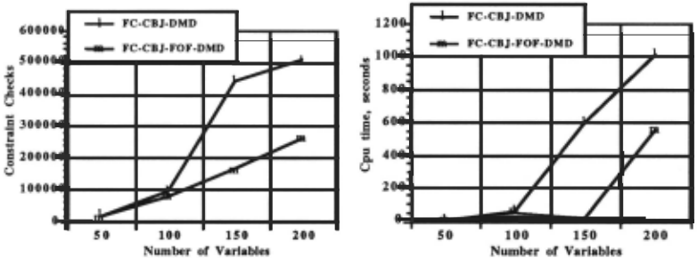
We do just this in the second experiment (Figure 5) taking off from the point where we obtained the best re sult in the first experiment. At this point the parameters were: a tightness of .675, 50 variables with 8 values, and a degree of 3.136. We keep these parameters fixed except for the number of problem variables, which we increase from 50, to 100, 150 and 200. (Our analysis suggests that by maintaining a fixed degree, as opposed to a fixed den sity, we will in theory remain on the hard problem ridge.) In this experiment we restrict our attention to the two best algorithms from the first experiment. The savings become quite significant.
So far, although our generator allows some variation, we have been lookly at basically homogeneous random problems. One might expect that application problems would involve more heterogeneity in their structure. In the third experiment we introduced more divergence in structure by removing or loosening constraints. We started with a set of 5 "ridge" problems with 99 vari ables, a domain size of 4, tightness .25 and density .06. (This density corresponds to an average degree of ap proximately 7.75.) For each of these we generated a se quence of problems by randomly choosing variables, five at a time, with degree greater than 3, and reducing their degree to three (by randomly removing constraints in volving the variables). We call this process introducing weak spots into the problem. Figures 6a-e shows these five problem sequences. (Note that the scales differ.) In Figure 6f we induce weak spots (in the problem of Figure 6a) in a different manner, by loosening the constraints around variables rather than removing them (so that the tightness times the degree is less than 1).
| FC-DMD | FOF-DMD | FC-CBJ-DMD | FC-CBJ-FOF-DMD | ||
|---|---|---|---|---|---|
| tightness | .150 | 11,299,439 | 11,476,507 | 11,054,443 | 10,957,579 |
| density | .450 | (319.0) | (798.1) | (1,800.4) | (1,897.2) |
| tightness | .325 | 2,559,008 | 2,177,734 | 2,288,183 | 1,900,228 |
| density | .150 | (232.9) | (258.3) | (488.3) | (448.3) |
| tightnes | .500 | 406,959 | 282,016 | 257,849 | 194,229 |
| density | .065 | (45.8) | (41.7) | (51.3) | (43.4) |
| tightness | .675 | 437,418 | 45,230 | 20,351 | 14,347 |
| density | .025 | (49.6) | (8.6) | (5.0) | (3.8) |
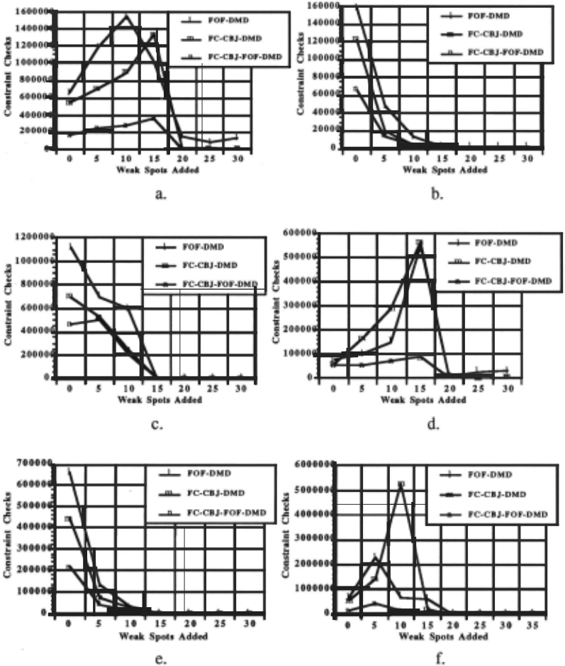
We do not show the FC-DMD results; in the first problem for example FC-DMD peaks at close to 50 mil lion constraint checks, way off the chart shown in Figure 6a. Our IDC algorithm was tested on these problems in [Freuder and Hubbe 93]; FOF-DMD actually performs somewhat better. (IDC has not been combined with FC-CBJ.)
The general lesson of these figures seems to be that CBJ and FOF complement each other nicely in coping with the induced inhomogeneity. The weak spots may also hinder standard forward checking, by reducing the pruning that forward checking can accomplish. This may lead to larger failed subproblems, which in turn provide an opportunity for FOF. Although we did not design these problem sequences specifically for FOF, these ap proaches to inducing inhomogeneity would admittedly appear to favor FOF. However, the larger point is that in inhomogeneous problems with a range of degrees and tightnesses there may well be areas with a structure for which FOF is particularly well suited, and FOF seems well able to take advantage of such local opportunities.
5 Potential
As the IDC algorithm demonstrates, a primary potential application of the extraction method arises in situations where we can determine that a subproblemS has no so lution, or does not have all the solutions - S can then be discarded. We might know S has no solutions from pre vious experience, e.g. with a similar problem. We might infer it from domain knowledge. The coloring problem illustration used in the first section is an example. We can "create" unsolvable subproblems. Take any inconsis tent pair of values a and b for X and Y. The subproblem obtained by reducing the domain of X andY to a and b, can be factored out. Taking this further: if the sets of values A for X and B for Y are such that no pair of values from A and B is consistent we can factor out the larger subproblem where X and Y are only reduced to A and B. We could look for pairs of value subsets, A and B, which are optimal in the sense that any pair of values in their Cartesian product is inconsistent, and no other pair of value subsets produces a larger Cartesian prod uct in which all value pairs are inconsistent. Optimal pairs are probably too hard to find, but we might have heuristics for finding good ones. (Contrast this approach with the work in [Hubbe and Freuder 92], which utilizes the Cartesian product of consistent pairs of values.) To some degree we are trying to "extract" the tight con straint, or part of it. This may in some sense loosen the A-B constraint, making it perhaps more likely that what remains will succeed.
Call a subproblem, S, involving some of the values, for some, but not all, of the variables, a subset, subdomain subproblem. S extends to a subdomain subproblem, S' involving all of the variables, in which the domains of the variables not in S are not reduced at all. Call S' the extension of S. If S is unsolvable, its extension will be also. If we can identify an unsolvable subset, sub domain subproblem we can factor out its extension. As an illustration we can generalize the earlier coloring ex ample. 3-cliques (triangles) cannot be colored with 2 colors. For every 3-clique we can factor out a subprob lem where 3 variables have the same 2 colors and the rest of the variables have all possible colors. Another simple illustration: in the n-queens problem, a subprob lem that includes a 3-queens problem cannot be solved. For example, consider a subproblem in which the first three rows are restricted to take values from the first three columns.
Alternatively, we can extract subproblems that we sus pect have solutions. This will enable us to focus on such subproblems early. If we know that a subset, subdomain subproblem S does have a solution, we can extract its extension. We are not guaranteed the extension has a solution, but it might be a good place to look. If we know an actual solution for S we can extract a subprob lem where the values for the S variables are the solution and all values are available again for variables not in S. Again, this might be a good place to look. This idea can be extended if we have the Cartesian product represen tation of a set of solutions [Hubbe and Freuder 1992], where each tuple in the Cartesian product is a solution. Again we can extract a subproblem where the values for the S variables are the values in the Cartesian product set, and all values are available for variables not in S. To some degree here we can again try to "extract" a tight constraint (or several of them), but this time by consid ering a subproblem where the only values remaining for the variables involved form a Cartesian product set of solutions. Since all pairs are possible in the subproblem the constraint is effectively eliminated.
The extraction method could also be useful if we have other reasons to want to work on S first (or last), ear lier (or later), in the search for a solution. We might even wish to factor out a subproblem that contains pos sibilities that are not considered to be of interest at the moment, or alternatively embody current preferences. Another way to get good subproblems to try first might be to extract a subproblem where all the values were loosely constraining and/ or constrained. Ideally this would mean loose within the subproblem, as opposed to within the problem as a whole, but that seems harder to achieve. For example we might collect the values that relatively speaking are most consistent with other values in each domain and extract that subproblem to work on first. Notice that this is related to, but not equivalent to, the idea of value ordering for "succeed first". Our scheme allows us to try all the "easiest" combinations before we involve any of the less likely values, and still know exactly what we left out, in case we do not find a solution with these values, or want to look for more solutions. Alternatively we could try to recognize good subproblems to put off examining, by extracting sub problems where all the values were tightly constraining and/or constrained. Or we could try to be more sophis ticated yet about identifying subproblems with charac teristics that strongly suggest the existence or absence of solutions.
Work on "really hard" problems has provided con siderable insight in this regard [Cheeseman et al. 91, Williams and Hogg 92], which has been tested on various types of CSPs. Likelihood of solution has been related to the tightness and density of constraints. Likelihood of solution has also been related to problem difficulty. Re ally hard problems have often been found on a "ridge" in "tightness/density space" between a region where prob lems are very likely to have solutions and a region where they are very likely to be unsolvable. We could try to extract in such a way so as to move pieces of the problem outside these really hard problem parameters, by trying to raise or lower constraint tightness. Starting with an overall hard problem we might try to extract subprob lems that were not hard or isolate the hard part of a problem in a smaller subproblem. This strategy might be particularly useful for inhomogeneous problems.
Constraint density could also be adjusted. Earlier we considered extracting subproblems in which all pairs of values between some variables were consistent. If the domains of X and Y in the subproblem consist only of mutually consistent values then there is effectively no constraint left between X and Yin the subproblem and it can be deleted. Following up on this notion of "eliminat ing constraints" in subproblems, we can try to extract out subproblems with desirable structure. By deleting enough constraints in this way we can try to reduce to a tree or 2-tree, for example [Freuder 90].
Note that the factoring out decomposition can be applied recursively. For example, we might try 3coloring hard graphs, factoring out 3-cliques, and doing some "forward checking" -type local consistency process ing whenever a domain is reduced to 1 element in a sub problem [Nadel 89]. We have seen how the factoring out process can be applied repeatedly during search. Extrac tion may prove particularly useful for dynamic CSPs, or "families" of related CSPs (where we have information about subproblems left over from previous experience) and for inhomogeneous CSPs (where we can extract hard or easy pieces). (We need to consider overhead of course, but some required information may come "free". The FOF decomposition uses only the constraint checks nor mally performed by forward checking.)
Our extraction mechanism provides an opportunity for practitioners to utilize domain-specific knowledge about subproblems. This knowledge may be available a priori, such as the simple "theorem" about uncolorable sub problems used in Section 1, or it may be acquired knowl edge. The acquired knowledge may be obtained and used while solving a single problem, as is the knowledge used by FOF, or it might be acquired while solving an ini tial set of problems and then applied to enhance future performance in the same domain.
6 Conclusion
We have introduced a general method for disjunctively decomposing a constraint satisfaction problem so that one of the resulting subproblems will be any specified subdomain subproblem. We suggested a number of uses for this decomposition and implemented and tested one that factors out unsolvable subproblems discovered dur ing search.
Acknowledgements
We wish to thank Gerard Verfaillie for pointing out to us that IDC decomposition generalizes to subdomain sub problem extraction and for further helpful discussion.
@inproceedings{ijcai1995p72,
  title     = {Extracting Constraint Satisfaction Subproblems},
  author    = {Freuder, Eugene C. and Hubbe, Paul D.},
  booktitle = {Proceedings of the Fourteenth International Joint Conference on
               Artificial Intelligence, {IJCAI-95}},
  publisher = {International Joint Conferences on Artificial Intelligence},
  editor    = {Chris S. Mellish},
  pages     = {548--556},
  year      = {1995},
  note      = {Constraint Satisfaction},
  url       = {https://ijcai.org/proceedings/1995/72},
}
TY - CPAPER TI - Extracting Constraint Satisfaction Subproblems AU - Freuder, Eugene C. AU - Hubbe, Paul D. T2 - Proceedings of the Fourteenth International Joint Conference on Artificial Intelligence, IJCAI-95 PB - International Joint Conferences on Artificial Intelligence PY - 1995 SP - 548 EP - 556 UR - https://ijcai.org/proceedings/1995/72 ER -Copied
Machine-readable versions of this paper, for tools and AI agents:





