A Theoretical Evaluation of Selected Backtracking Algorithms

1 Introduction

Constraint-based reasoning is a simple, yet powerful paradigm in which many interesting problems can be formulated. It has received much attention recently, and numerous methods for dealing with constraint networks have been developed. The applications include graph coloring, scene labelling, natural language parsing, and temporal reasoning.

The basic notion of constraint-based reasoning is a con­ straint network, which is defined by a set of variables, a do­ main of values for each variable, and a set of constraints between the variables. To solve a constraint network is to find an assignment of values to each variable so that all constraints are satisfied.

Backtracking search is one of the methods of solving con­ straint networks. The generic backtracking algorithm was first described more than a century ago, and since then has been rediscovered many times [Bitner and Reingold, 1975]. In recent years, many new backtracking algorithms have been proposed. The basic ones include Backmark­ ing [Gaschnig, 1977], Backjumping [Gaschnig, 1978], For­ ward Checking [Haralick and Elliot, 1980], and Conflict­ Directed Backjumping [Prosser, 1993]. Several hybrid al­ gorithms, which combine two or more basic algorithms, have also been developed [Prosser, 1993].

·currently with MPR Teltech Ltd, Burnaby, BC, Canada

There is no simple answer to the question which back­ tracking algorithm is the best one. First, the performance of backtracking algorithms depends heavily on the problem being solved. Often, it is possible to construct exam~les of constraint networks on which an apparently very efficient algorithm is outperformed by the most basic chronological backtracking. Second, it is not obvious what measure should be employed for comparison. Run time is not a very reliable measure because it depends on hardware and implementa­ tion, and so cannot be easily reproduced. Besides, the cost of performing consistency checks (checks that verify that the current instantiations of two variables satisfy the constraints) cannot be determined in abstraction from a concrete problem. A better measure of the efficiency of a backtracking algorithm seems to be the number of consistency checks performed by the algorithm, although it does not account for the overhead costs of maintaining complex data structures. Another stan­ dard measure is the number of nodes in the backtrack tree generated by an algorithm.

The need for ordering algorithms according to their effi­ ciency has been recognized before. Nudel [1983] ordered backtracking algorithms according to their average-case per­ formance. Prosser [1993] performed a series of experiments to evaluate nine backtracking algorithms against each other. However, such an approach is open to the criticism that the test problems are not representative of the problems that arise in practice. Even a theoretical average-case analysis is pos­ sible only if one makes simplifying assumptions about the distribution of problems. Prosser commented on his results:

It is naive to say that one of the algorithms is the 'champion'. The algorithms have been tested on one problem, the ZEBRA. It might be the case that the relative performance of these algorithms will change when applied to a different problem.

When Prosser's results are examined, it is easy to notice that in some cases one algorithm performed better than another in all tested instances. Could this mean that one algorithm is always better than another? Such a hypothesis can never be verified solely by experimentation; the relationship has to be proven theoretically. In this paper we show that some of these cases indicate a general rule, whereas other do not. More­ over, we present a partial ordering of several backtracking algorithms which is valid for all instances of all constraint satisfaction problems.

Our approach is purely theoretical. We analyze several backtracking algorithms with the purpose of discovering gen­ eral rules that determine their behaviour. A notion of incon­ sistency between instantiations and variables is introduced, and is shown to be a useful tool for characterizing such well­ known concepts as backtrack, backjump, and domain annihi­ lation. Using the new notion, we formulate the necessary and sufficient conditions for a search tree node to be visited by each backtracking algorithm. These characterizations enable us to construct partial orders (or hierarchies) of the algorithms according to two standard performance measures: the num­ ber of visited nodes, and the number of performed consistency checks.

The orderings are surprisingly regular and contain some non-intuitive results. For instance, it turns out that the set of nodes visited by Forward Checking is always a subset of the set of nodes visited by Backjumping. This fact has never been reported before although the two algorithms have been often empirically compared. Also, the orderings confirm and clar­ ify the experimental results published by other researchers. The characterizing conditions imply simple and elegant cor­ rectness proofs of the characterized algorithms. Two of these algorithms, Backjumping (BJ) and Conflict-Directed Back­ jumping (CBJ) have not been formally proven correct before 1 .

The orderings proved also to be a stimulus for developing more efficient backtracking algorithms. The idea of combin­ ing Backjumping and Backmarking into a new hybrid algo­ rithm was first put forward by Nadel [1989]. Such algorithm, called BMJ, was presented by Prosser [ 1993]. BMJ, however, does not retain all the power of both base algorithms in terms of consistency checks. Prosser observed that on some in­ stances of the zebra problem BMJ performs more consistency checks than BM. In the conclusion of his paper he posed the following question:

It was predicted that the BM hybrids, BMJ and BM-CBJ, could perform worse than BM because the advantages of backmarking may be lost when jumping back. Experimental evidence supported this. Therefore, a challenge remains. How can the backmarking behaviour be protected?

In this work we answer the question by modifying the two BM hybrids, Backmarking with Backjumping (BMJ), and Back­ marking with Conflict-Directed Backjumping (BM-CBJ), so that they always perform fewer consistency checks than both corresponding basic algorithms.

Apart from presenting specific results for particular back­ tracking algorithms, our goal is also to propose a general methodology: techniques and definitions that can be used for characterizing any backtracking algorithm. This kind of the­ oretical analysis may be performed for any new backtracking algorithm in order to see if it belongs in the existing hierarchy.

1 Both BJ and CBJ were first presented without correctness proofs and no direct proofs of these algorithms have appeared in the literature. However, proofs have been given for certain algo­ rithms related to BJ and CBJ [Bruynooghe, 1981 ; Ginsberg, 1993; Schiex and Verfaillie, 1994].

2 Background

We begin with some concepts of the constraint satisfaction paradigm, then give a brief description of four basic back­ tracking algorithms, and finally present an example that shows the algorithms at work.

Definition 1 A binary constraint network [Montanari, 1974] consists of a set of n variables { x 1 , .. . , x n}; their respective value domains, D1, · · · , Dn; and a set of binary constraints. A binary constraint or relation, R;j. between variables x; and Xj, is any subset of the product of their domains 2 (that is, R;i ~ D; x Dj ). We denote an assignment of values to a subset of variables by a tuple of ordered pairs, where each ordered pair ( x, a) assigns the value a to the variable x. A tuple is consistent if it satisfies all constraints on the variables contained in the tuple. A (full) solution of the network is a consistent tuple containing all variables. A partial solution of the network is a consistent tuple containing some variables. For simplicity, we usually abbreviate ( ( x1, a1 ) , .. . , ( x; , a;))) to (a 1 , · ·· , a;).

The next definition introduces a notion of consistency be­ tween a tuple of instantiations and a set of variables. This notion is fundamental to all results presented in this work.

Definition 2 A tuple ((x; 1 , a; 1 ) , ··· , (x;u , a;J) is consistent with a set of variables {xi 1 , · ·· , xi.} if there exist instanti­ ations a it , . . . , ai. of the variables x it, . .. , xi. respectively, such that the tuple ((x;t> a; 1 ) , ··· , (x;u , a;J , (xit> ait) , . .. , (xi., ai.)) is consistent. A tuple is consistent with a vari­ able if it is consistent with a one-element set containing this variable.

The idea of a backtracking algorithm is to extend partial solutions. At every stage of backtracking search, there is some current partial solution which the algorithm attempts to extend to a full solution. Each variable occurring in the current partial solution is said to be instantiated to some value from its domain. In this work we assume the static order of instantiation in which variables are added to the current par­ tial solution according to the predefined order: x 1, . . . , Xn. It is convenient to divide all variables into three sets: past variables (already instantiated), current variable (now being instantiated), and future variables (not yet instantiated). A dead-end occurs when all values of the current variable are rejected by a backtracking algorithm when it tries to extend a partial solution. In such a case, some instantiated variables become uninstantiated; that is, they are removed from the current partial solution. This process is called backtracking. If only the most recently instantiated variable becomes unin­ stantiated then it is chronological backtracking. Otherwise, it is backjumping. A backtracking algorithm terminates when all possible assignments have been tested or a certain number of solutions have been found.

A backtrack search may be seen as a search tree traversal. In this approach we identify tuples (assignments of values to variables) with nodes: the empty tuple f is the root of the tree, the first level nodes are !-tuples (representing an assignment of a value to variable x1), the second level nodes are 2-tuples, and so on. The levels closer to the root are called lower levels, and the levels farther from the root are called higher levels. Similarly, the variables corresponding to these levels are called lower and higher. The nodes that represent consistent tuples are called consistent nodes. The nodes that represent inconsistent tuples are called inconsistent nodes. We say that a backtracking algorithm visits a node if at some stage of the algorithm's execution the instantiation of the current variable and the instantiations of the past variables form the tuple identified with this node. The nodes visited by a backtracking algorithm form a subset of the set of all nodes belonging to the search tree. We call this subset, together with the connecting edges, the backtrack tree generated by a backtracking algorithm. Backtracking itself can be seen as retreating to lower levels of the search tree. Whenever some variables become uninstantiated and x h is set as the new current variable, we say that the algorithm backtracks to level h. We consider two backtracking algorithms to be equivalent if on every constraint network they generate the same backtrack tree and perform the same consistency checks.

2 Throughout the paper we assume that all domain values satisfy the corresponding unary constraints.

Chronological Backtracking (BT) [Bitner and Reingold, 1975] is the generic backtracking algorithm. The consistency checks between the instantiation of the current variable and the instantiations of the past variables are performed according to the original order of instantiations. If a consistency check fails, the next domain value of the current variable is tried. If there are no more domain values left, BT backtracks to the most recently instantiated past variable. If all checks succeed, the branch is extended by instantiating the next variable to each of the values in its domain. A solution is recorded every time when all consistency checks succeed after the last variable has been instantiated.

Backjumping (BJ) [Gaschnig, 1978] is similar to BT, ex­ cept that it behaves more efficiently when no consistent in­ stantiation can be found for the current variable (at a dead­ end). Instead of chronologically backtracking to the preceding variable, BJ backjumps to the highest past variable that was checked against the current variable.

Conflict-Directed Backjumping (CBJ) [Prosser, 1993] has a more sophisticated backjumping behaviour than BJ. Every variable has its own conflict set that contains the past variables which failed consistency checks with its current instantiation. Every time a consistency check fails between the instantiation a; of the current variable and some past instantiation ah, the variable xh is added to the conflict set of x;. When there are no more values to be tried for the current variable x;, CBJ backtracks to the highest variable Xh in the conflict set of x;. At the same time, the conflict set of x ; is absorbed by the conflict set of x h, so that no information about conflicts is lost.

In contrast with the above backward checking algorithms, Forward Checking (FC) [Haralick and Elliot, 1980] performs consistency checks forward, that is, between the current vari­ able and the future variables. After the current variable has been instantiated, the domains of the future variables are fil­ tered in such a way that all values inconsistent with the current instantiation are removed. If none of the future domains is annihilated, the next variable becomes instantiated to each of the values in its filtered domain. Otherwise the effects of for­ ward checking are undone, and the next value is tried. Ifthere are no more values to be tried for the current variable, FC backtracks chronologically to the most recently instantiated variable. A solution is recorded every time the last variable becomes instantiated.

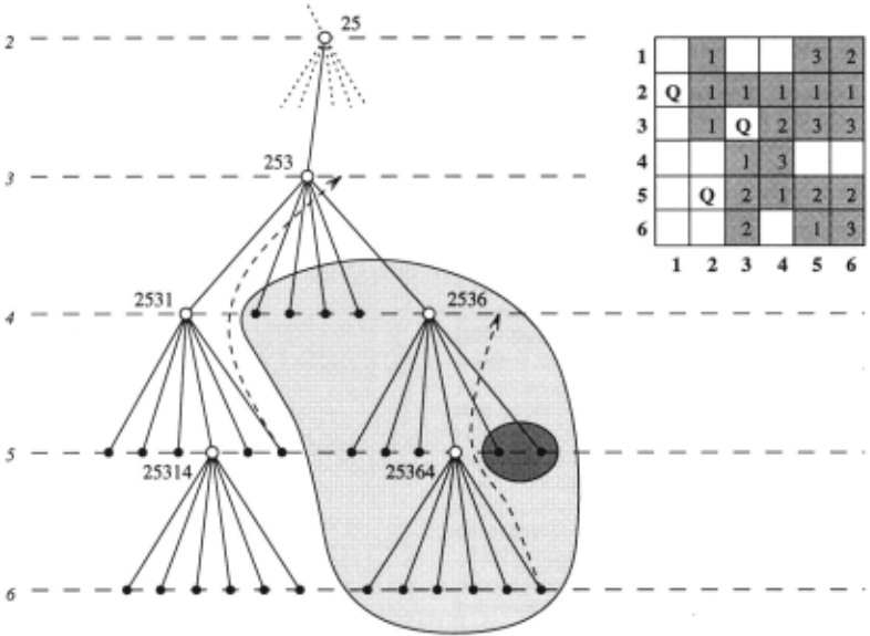
Example 1. The n-queens problem is how to place n queens on a n x n chess board so that no two queens at­ tack each other. Our representation of this problem identifies board columns with variables, and rows with domain values. Figure 1 shows a fragment of the backtrack tree generated by Chronological Backtracking (BT) for the 6-queens problem. White dots denote consistent nodes. Black dots denote incon­ sistent nodes. For simplicity, when referring to nodes we omit commas and parentheses. The board in the upper right corner depicts the placing of queens corresponding to node 253 in the backtrack tree. Capital Q's on the board represent queens which have already been placed on the board. The shaded squares represent positions that must be excluded due to the already placed queens. The numbers inside the squares indi­ cate the queen responsible for the exclusion; I ,2,3 correspond to the first, second, and third queen respectively.

The dark-shaded part of the tree contains two nodes that are skipped by Backjumping (BJ). The algorithm detects a dead­ end at variable x6 when it tries to expand node 25364. It then backjumps to the highest variable in conflict with X6, in this case x4. The backjump is represented by a dashed arrow. We could say that BJ discovers that the tuple (2,5,3,6), which is composed of instantiations in conflict with X6, is inconsistent with variable x6. To see this, notice that if we place a queen in column 4 row 6, every square in column 6 is attacked by the queens placed in the first four columns. Indeed, there is no point in trying out the remaining values for xs because that variable plays no role in the detected inconsistency. Nodes 25365 and 25366 may be safely skipped.

The light-shaded part of the tree contains nodes that are skipped by Conflict-Directed Backjumping (CBJ). The algo­ rithm reaches a dead-end when expanding node 25314. At this moment the conflict set of x6 is { 1, 2, 3, 5} because the instantiations of these four variables prevent a consistent in­ stantiation of variable X6 . To see this, notice that after the fourth and the fifth queen are placed, column 6 of the chess board will contain numbers 1, 2, 3, and 5. CBJ backtracks to the highest variable in the conflict set, which is xs. No nodes are skipped at this point. The conflict set of X6 is absorbed by the conflict set of xs, which now becomes {I , 2, 3}. After trying the two remaining values for x5, CBJ backjumps to x3 skipping the rest of the subtree. The back jump is represented by a dashed arrow. In terms of consistency, we could say that the algorithm discovered that tuple (2,5,3) is inconsistent with the set of variables { x5 , x6}. A look at the board in Figure I convinces us that indeed such a placement of queens cannot be extended to a full solution. It is impossible to fill columns 5 and 6 simply because the two available squares are in the same row. Note that (2,5,3) is consistent with both xs and X6 taken separately.

Forward Checking (FC), in contrast with the backward checking algorithms, visits only consistent nodes, although not necessarily all of them. In our example, nodes 253, 2531, 25314 and 2536 are visited, but not 25364. The board in Figure 1 can be interpreted in the context of this algorithm as follows. The shaded numbered squares correspond to the values filtered from domains of variables by forward check­ ing. The squares that are left empty as the search progresses correspond to the nodes visited by FC. Due to the filtering scheme, FC detects an inconsistency between the current par­ tial solution and some future variable without ever reaching that variable, but it is unable to discover an inconsistency with a set of variables. In our example, the algorithm finds that both 25314 and 2536 are inconsistent with x6. However, it does not discover that node 253 is inconsistent with { xs, x6}. That is why node 2536 is visited by FC even though it is skipped by the backward checking CBJ.

3 Characterizations and Their Implications

We are now ready to present some new results. First, we give two lemmas that define backjumps in terms of inconsistency between variables and instantiations. Then, we present theo­ rems about the backtrack trees of the four basic backtracking algorithms: BT, BJ, CBJ, and FC. The theorems enable us to (a) partially order the algorithms according to the number of visited nodes, and (b) prove the correctness of the algo­ rithms. It is assumed that all constraints are binary, the order of instantiations is fixed and static, and the order of perform­ ing consistency checks within the node follows the order of instantiations. We deal with the more general problem of finding all solutions; at the end of the section we briefly com­ ment on the validity of our results when only one solution is sought. The proofs that are not included here can be found in [Kondrak, 1994].

Lemma 1 If BJ backtracks to variable x h from a dead-end at variable x; then ( a 1, ·.. , a h) is inconsistent with x;.

Proof After no consistent instantiation can be found for x;, BJ chooses as the point of backtrack the variable x h which is the highest variable in conflict with x;. Let C; denote the tuple composed of instantiations of all variables that are in conflict with x;. Clearly, C; is inconsistent with x;. Since ah is the instantiation of the highest variable in C;, C; is a subtuple of (a1, ... , ah)· Therefore, (a1, ... , ah) is also inconsistent with X;. 0

Lemma 2 If CBJ backtracks from variable x; to variable xh then C; is inconsistent with S, where C; is the tuple composed of instantiations of the variables in the conflict set of x;, and S isasubsetof{x;, ... ,xn} containingx;.

The following theorem specifies the sufficient conditions for a node to be visited by the four basic backtracking algo­ rithms.

Theorem 1

1. BT visits a node if its parent is consistent.
2. BJ visits a node if its parent is consistent with all vari­ ables.
3. CBJ visits a node if its parent is consistent with all sets of variables.
4. FC visits a node if it is consistent and its parent is con­ sistent with all variables.

Proof

1. Suppose that node ( a1, .. . , a;_ 1) is consistent with all variables, and its child p = ( a1, ·.. , a;) is not visited by BJ. Take the highest j such that node p' = (a 1 , . . . , ai) is visited by BJ. Node p' is a proper ancestor of node p and

is consistent with all variables. When BJ is at node p', all consistency checks between ai and previous instan­ tiations succeed. The only reason for not instantiating the next variable Xj+l to ai+l can be a backjump from some variable x h to some variable x 9 , where g ~ j and h 2: j + 2. But if this is the case, Lemma 1 implies that node (a 1, ··. , a 9 ) is inconsistent with x h, which contra­ dicts the initial assumption that node (at, ... , a;-t) is consistent with all variables.

1. Similar to the proof of b), except that we use Lemma 2. Proofs of the remaining cases are straightforward. D

The next theorem specifies the necessary conditions for a node to be visited by the four backtracking algorithms.

Theorem 2

1. BT visits a node only if its parent is consistent.
2. BJ visits a node only if its parent is consistent.
3. CBJ visits a node only if its parent is consistent.
4. FC visits a node only if it is consistent and its parent is consistent with all variables.

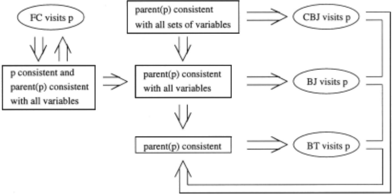
Figure 2 summarizes the results presented so far. The arrows represent implications formulated in Theorems 1 and 2. Note the difference between the chronologically backtracking al­ gorithms BT and FC, and the backjumping algorithms BJ and CBJ. The former are completely characterized as the neces­ sary and sufficient conditions coincide; for every node we can decide whether it is visited by the algorithm without gener­ ating the whole backtrack tree. The latter are only partially characterized; there is a set of nodes for which we are unable to tell a priori if they belong to the algorithm's search tree or not. It is an open question if better characterizing conditions for the backjumping algorithms can be found.

The following corollary has been formulated by simply following the arrows in Figure 2.

Corollary 1

1. BT visits all nodes that BJ visits.
2. BT visits all nodes that CBJ visits.
3. BT visits all nodes that FC visits.
4. BJ visits all nodes that FC visits.

The relationship between BJ and FC is the most interesting. It has never been reported before, although the two algorithms have been often empirically compared.

A relationship between BJ and CBJ, although not implied by the theorems, can also be proven using Lemmas 1 and 2.

Theorem 3 BJ visits all nodes that CBJ visits.

Corollary 1 together with Theorem 3 enable us to construct a partial order of backtracking algorithms with respect to the number of visited nodes. BT generates the largest backtrack tree, which contains all nodes visited by the other algorithms. BJ visits more nodes than CBJ or FC. The order would be linear if there was a relationship between FC and CBJ, but this is not the case. Figure 1 provides a counterexample: some nodes visited by CBJ are not visited by FC, and vice versa.

The correctness of the four basic algorithms is also an al­ most immediate consequence of the theorems. A backtrack­ ing algorithm is correct if it is sound (finds only solutions), complete (finds all solutions), and terminates. That all the algorithms terminate is clear, so only soundness and com­ pleteness have to be shown.

Corollary 2

1. BT is correct.
2. BJ is correct.
3. CBJ is correct.
4. FC is correct.

Proof

1. Soundness. A solution is claimed by BJ if all consistency checks succeed at an n-level node. This means that (at, ... , an) is visited and Vi < n : a; is consistent with an. Theorem 2 implies that its parent (at, ... , an-I) is consistent. Therefore, (a 1 , ... , an) is consistent.

Completeness. Suppose that some n-level node (at, ... , an) in the search tree is consistent. Then, its parent (a 1, . .. , an- 1) is consistent as well, and it is also consistent with Xn . Therefore, (a1, .. . ,an-I) is con­ sistent with all variables. From Theorem I we know that (a 1, ... , an) is visited by BJ. Since all consistency checks between an and previous instantiations must suc­ ceed, a solution is claimed by BJ.

Proofs of the remaining cases are similar. D

Naturally, our approach can be extended to other backtrack­ ing algorithms.

All the above results were originally proven with the as­ sumption that the search is not interrupted until all possibilities are exhausted. This is not generally true if only a fixed number of solutions is sought. However, if we restrict our attention to only those of the search tree nodes that precede (in the preorder traversal) the last node visited by a backtracking al­ gorithm, the theorems are still valid. Therefore, our results hold also for the "one solution" versions of the backtracking algorithms, with only slightly modified proofs.

4 Hybrid Algorithms with Backmarking

In this section we briefly discuss Backmarking [Gaschnig, 1977] and its two hybrids. We propose a modification to the hybrids, and then include these algorithms in our hierarchies.

Backmarking (BM) imposes a marking scheme on the Chronological Backtracking algorithm in order to eliminate some redundant consistency checks. The scheme is based on the following two observations [Nadel, 1989]: (a) If at the most recent node where a given instantiation was checked the instantiation failed against some past instantiation that has not yet changed, then it will fail against it again. Therefore, all consistency checks involving it may be avoided. (b) If, at the most recent node where a given instantiation was checked, the instantiation succeeded against all past instantiations that have not yet changed, then it will succeed against them again. Therefore we need to check the instantiation only against the more recent past instantiations which have changed.

The marking scheme is implemented using two arrays: mbl (minimum backup level) of size n, and mel (maximum check­ ing level) of size n x m. The entry mbl[i] contains the number of the lowest variable whose instantiation has changed since the variable x; was last instantiated with a new value. The entry mcl[i)[j) contains the number of the highest variable that was checked against the j-th value in the domain of the variable x;.

Nadel [1989] suggested combining BM and BJ into a new hybrid algorithm. Prosser presented such algorithm, called Backmarking and Backjumping (BMJ), in [Prosser, 1993]. BMJ, however, does not retain all the power of each base algorithm in terms of consistency checks. Prosser observed that on some instances of the zebra problem BMJ performs more consistency checks than BM. BMJ is also worse than BM on the benchmark 8-queens problem.

A careful analysis of the algorithm leads us to the conclu­ sion that BMJ is sometimes worse than BM because the mbl array, which was originally designed for a chronologically backtracking algorithm, is no longer adequate for a back­ jumping algorithm. Since BM always tests all values of the current variable for consistency, a single entry for all values is sufficient. In BMJ, however, it often happens that only some values of the current instantiation are tested, and the other values are skipped by a backjump. A separate entry for each value is therefore necessary to preserve all collected consistency information.

We propose a modified BackMarkJump (BMJ2), which solves the problem by making mbl a two-dimensional rather than a one-dimensional array. The new mb/ array is of size n x m, where n is the number of variables, and m is the size of the largest domain. This is a reasonable space requirement because BMJ already uses one n x m array; each me/ entry has now a corresponding mb/ entry. The mbl[ i] [j) entry stores the number of the lowest variable whose instantiation has changed since the variable x; was last instantiated with the j-th value. The entry is set to i every time the current instantiation ( x; , t i) is being tested for consistency with past instantiations. When the algorithm backtracks, the entries are updated in a similar way as in BMJ. Thanks to the more efficient backmarking scheme BMJ2 is always better than BMJ. Moreover, since BMJ2 does not lose information about consistency checks in the way BMJ does, it is always better than BM.

An analogous modification of Backmarking and Conflict­ Directed Backjumping (BM-CBJ), which is another hybrid proposed by Prosser, produces BM-CBJ2: mbl should be made a 2-dimensional array, and maintained in the same way as in BMJ2.

5 Hierarchies

We now present two hierarchies, which include the four ba­ sic backtracking algorithms described in Section 2, and the Backmarking hybrids discussed in Section 4.

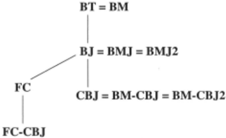
The hierarchy with respect to the number of visited nodes is presented in Figure 3. Two algorithms are connected by a link if the set of nodes visited by one of them is always a subset of the set of nodes visited by the other. Naturally, the relation is transitive. The relationships derived in Section 3 form the core of the hierarchy. Note that imposing a backmarking scheme on an algorithm does not change the set of nodes that are visited. Thus, for example, BM generates exactly the same backtrack tree as BT.

Figure 4 shows the hierarchy of algorithms with respect to the number of consistency checks. Two algorithms are connected by a link if one of them always performs no more consistency checks than the other. Since BT, BJ, and CBJ perform the same number of consistency checks at any given node, they are in the same order as in the nodes hierarchy. Im­ posing a marking scheme on a backtracking algorithm results in a reduction of the number of consistency checks performed. The figure contains also one Forward Checking hybrid: For­ ward Checking and Conflict-Directed Backjumping (FC-CBJ) [Prosser, 1993], which has not been discussed here. For a treatment of FC-CBJ see [Kondrak, 1994].

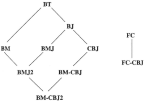
Besides the relationships that are shown explicitly, it is important to note the ones that are implicit in the picture. In order to disprove a relationship between A and B, one needs to find at least one constraint satisfaction problem on which A is better than B, and one on which B is better than A . For example, BM performs fewer consistency checks than FC on the regular 8-queens problem, but more on the confused 8-queens problem [Nadel, 1989]. Examples of constraint networks were found that disprove all relationships that are not included in the hierarchies. Thus, however counterintuitive it may seem, FC-CBJ may visit more nodes than CBJ, and perform more consistency checks than BT.

6 Conclusions

We presented a theoretical analysis of several backtracking al­ gorithms. Such well-known concepts as backtrack, backjump, and domain annihilation were described in terms of inconsis­ tency between instantiations and variables. This enabled us to formulate general theorems that fully or partially describe sets of nodes visited by the algorithms. The theorems were then used to prove the correctness of the algorithms and to con­ struct hierarchies of algorithms with respect to the number of visited nodes and with respect to the number of consistency checks. The gaps in the resulting hierarchy prompted us to modify existing hybrid algorithms so that they are superior to the corresponding basic algorithms in every case. One of the modified algorithms is always better (in terms of con­ sistency checks) than all six backward checking algorithms described by Prosser in [Prosser, 1993]. In the future the hier­ archies could be extended by applying our approach to other backtracking algorithms, such as Dechter's graph-based back­ jumping algorithm [Dechter, 1990] and Nadel's backtracking algorithm with full arc-consistency lookahead [Nadel, 1989].