Using Inferred Disjunctive Constraints To Decompose Constraint Satisfaction Problems

1 Introduction

Constraint satisfaction problems (CSPs) involve finding values for a set of problem variables consistent with a set of constraints on which combinations of , values are permitted. They arise often in artificial intelligence, in fields ranging from temporal reasoning to machine vision.

This paper proposes a new technique that utilizes inferred disjunctive constraints to guide decomposition of a CSP. The decomposition reduces the size of the problem. The technique was used in an algorithm that achieved up to an order of magnitude improvement on difficult problems when compared with one of the most successful algorithms in the literature. The advantage of the new technique often increased as problem difficulty increased. The technique appears particularly well suited to taking advantage of local "weak spots" in globally difficult problems.

The following observation expresses the key idea: Given a solvable problem and a value v for a variable V, if there is no solution involving v, then there must be a solution involving a value inconsistent with v.

The basic problem decomposition can be illustrated with a simple example. Suppose we have a problem where one of the variables, X, is constrained by one other variable Y. Suppose value a for X is not consistent with values b and c for Y, i.e. the combination (a b) and the combination (a c) are not allowed, but a is consistent with all other values. Suppose further that the domain of every variable, the set of possible values, is D; so a is consistent with D-{ b c} for Y.

*This material is based on work supported by the National Science Foundation under Grant No, IRI-9207633.

We claim that we can divide and conquer by reducing the problem to two subproblems. One subproblem will be the same as the original except the domain of X will be {a} and the domain of Y will be D-{b c}. The other subproblem will be the same as the original except the domain of X will be D-{a} and the domain of Y will be { b c}. Notice that we are pruning away a subproblem, where the domain of X is D-{a} and the domain of Y is D-{b c}, that may contain solutions. However, we shall see that we can guarantee that not all solutions are pruned away.

Section 2 further develops the basic decomposition technique, and proves that it will not lose all solutions. Section 3 embeds this technique in an algorithm for solving CSPs. Section 4 adds some important refinements to the decomposition and the algorithm. Section 5 investigates the potential of the technique analytically, Section 6 experimentally.

2 Decomposition

We will assume in this paper that we are dealing with binary CSPs, where constraints involve two variables, which we will say share the constraint. In a constraint graph a binary CSP is represented with vertices for variables and edges for constraints. If variables share a constraint the corresponding vertices share an edge in the constraint graph, and thus the variables are called neighbors.

The weak inferred disjunctive constraint (weak IDC) decomposition of problem P around value v for variable V consists of the following subproblems: The first subproblem, Sy, is the same asP except the domain of V is restricted to { v} and the domains of the other variables are restricted to values consistent with V. Then, for each variable Vi that is a neighbor of V, we form a subproblem, SVi. that will be the same asP except that the domain of V will be its domain in P minus v, and the domain of Vi will consist of those values inconsistent with v.

We will call the first subproblem, the precluded subproblem, because values are deleted using a preclusion process [Golumb and Baumert, I965], and the rest the neighbor subproblems. We will call a subproblem empty if any of its variable domains is empty.

This decomposition generalizes the basic insight presented in Section 1. It derives from the inferred disjunctive constraint: if there is a solution, either there is a solution containing v, or there is one not containing v, but containing a value inconsistent with v.

Theorem 1: If a problem P has a solution, given a weak inferred disjunctive constraint decomposition of P around any value v for any variable V, one of the subproblems will have a solution that is a solution to P.

Proof: Either P has a solution involving v for V, or it does not. If it does, that solution clearly will be a solution of the subproblem that contains v for V. (The removal of values inconsistent with v does not remove any solutions.) If it does not, then any solution must contain at least one value inconsistent with v for V. Let us say that for a solution s the inconsistent value is v' for variable V'. The subproblem SV' will contain the solution s. ·

Note that there may be solutions to P that are not solutions to any subproblem. Such solutions would neither contain v nor any values inconsistent with v. However, this does not matter if we do not require all the solutions.

3 Algorithm

The decomposition process can be imbedded in a CSP algorithm. We start with a very basic implementation.

Weak IDC Algorithm:

Stack <- (initial problem, empty solution)

Until Stack empty:

Pop (Problem, Solution) from Stack

If Problem has only one variable, U

then Exit with Solution plus value(s) of U else

Decompose around first value, v, in first variable, V

For each non-empty neighbor subproblem, N: Push (N, Solution) onto Stack

If the precluded subproblem, SV, is not empty then

SV <- SV minus V

Push (SV, Solution plus v) onto Stack

This algorithm conducts a depth-first search through a "decomposition tree". The root is the original problem. The children of a node are produced by decomposing around the first value, v, in the list of potential values for the first variable, V, in the list of variables for the parent problem. The precluded subproblem is reduced further by eliminating v. .

Children are always smaller than parents (with fewer values), thus each branch of the tree terminates (assuming fmite domains). Leaf nodes are identifiable as solvable (they involve only one variable, and any value for this variable can be combined with the stored Solution to form a complete solution to the problem) or unsolvable (they produce no non-empty children). Theorem I ensures that a solvable problem cannot produce only unsolvable leaf nodes.

The algorithm can be viewed as a combination of the standard forward checking algorithm [Haralick and Elliott, I980], and the decomposition process. The local inconsistency removal in the first subproblem corresponds to a forward checking step.

4 Refinements

4.1 Further Domain Reduction

Consider the decomposition of P around v for V. In SVi. for each neighbor Vi, we can reduce the domain of Vj, for all j<i, to the set of values consistent with v. We call the this decomposition that uses this further reduction the inferred disjunctive constraint (/DC) decomposition. We call the set of neighbor subproblems after this further reduction the excised subproblems.

Theorem 2: If a problem P has a solution, given an IDC decomposition of P around any value v for any variable V, one of the subproblems will have a solution that is a solution toP.

Proof: SV I, which remains unchanged from the weak IDC decomposition, considers all the possibilities that exclude v and include values for VI inconsistent with v. Thus values for VI inconsistent with v can be ignored in SVk for k>l. SV2. where the domain of VI is now reduced to the values consistent with v, considers all the possibilities that exclude v and include values for V2 inconsistent with v, except those where the value for VI is also inconsistent with v; but those were considered in SVI· Thus values for V2 inconsistent with v can be ignored in SVk for k>2. This line of reasoning carries on to establish the validity of the overall reduction. ·

4.2 Ordering Heuristics

The algorithm presents new opportunities for ordering heuristics: choosing a variable domain in which to look for a value to decompose around, choosing the value, choosing the order in which subproblems are placed on the stack, maintaining the subproblems on an ordered agenda rather than a stack.

The variable ordering heuristic we test below is based on a well-known heuristic that we will refer to here as dynamic minimal domain variable ordering. This is a variable ordering heuristic that chooses a variable to instantiate with minimal current domain size. It has proven especially effective with forward checking, where preclusion effects changes in the current domain size of variables [Haralick and Elliott, I980]. We will refer to the combination of forward checking and dynamic minimal domain variable ordering as the FC-D algorithm, and use it as a basis for comparison in Section 6.

We use this heuristic to a limited degree in conjunction with IDC. After taking a precluded subproblem (or the initial problem) off the stack, the variable V from which we choose a value to decompose around is a variable with minimal current domain size. Otherwise we will simply choose the first remaining uninstantiated variable to process next. Note that for the remainder subproblem, by choosing the ftrSt uninstantiated variable to process we automatically get the effect of minimal domain size ordering, as this first variable will be V, whose domain has just been reduced further in size while the other domains have remained unchanged. We will refer to our our ordering strategy for IOC as dynamic minimal domain precluding variable ordering.

We also experimented a bit with a simple, static value ordering scheme. The problem was preprocessed to obtain an inconsistency count for each value v: this is the total number of values for all other variables inconsistent with v. During search when choosing a value for a variable V, a value in the current domain of V with a minimal inconsistency count is chosen. Call this the inconsistency count value ordering heuristic. When we test it below we add the constraint checks required to compute the inconsistency counts into the total search effort.

4.3 Conservative Decomposition Strategies

When a problem P is popped from the stack we can choose not to perform an IDC decomposition. Instead, after choosing a value v for a variable V, we can decompose into only two subproblems. The first is the same precluded subproblem as in the IDC decomposition; it includes v and the values consistent with v. (As before in the context of the algorithm we can further reduce the subproblem by removing V, adding v to the associated solution.) The second, which we will call the remainder subproblem, is the same as P except that the domain of V excludes v. If we always decompose in this way we end up with a non­ standard description of the standard forward checking algorithm. Thus we call this decomposition the forward checking decomposition.

We identify two conditions under which we will choose this more conservative decomposition strategy, in effect reverting to forward checking in these two circumstances. (Note that if we always used the forward checking decomposition and our dynamic minimal domain precluding variable search order that we would have an algorithm equivalent to FC-D.)

The frrst condition is that the precluded subproblem is empty (one of the variable domains is empty). In this case we end up only putting one subproblem onto the stack, and taking it right back off. So, in effect, we simply move right on to consider the next value for V. We will term the principle of avoiding IDC decomposition when the precluded subproblem is empty the empty domain decomposition heuristic. Theorem 5 below implies that IDC decomposition will not reduce the problem more than forward checking decomposition when the precluded subproblem is empty.

The second condition under which we choose the simpler decomposition utilizes an estimate of the relative complexity of the subproblems produced by the IDC decomposition versus those produced by the forward checking decomposition.

Since both decompositions include the precluded subproblem, we compare the excised subproblems from the IOC decomposition with the remainder subproblem from the forward checking decomposition. The size of a problem, as measured by the number of possible value combinations, is a reasonable heuristic estimate of problem complexity here, and is obtained by simply multiplying the domain sizes for the variables. The size of the remainder subproblem is compared with the sum of the sizes of the excised subproblems. (Actually we use the "consistent subproblem", defined below, to simplify the computations.)

We will show below that the former will in fact never be smaller. However, it proved desirable only to choose the IDC decomposition when the latter is smaller than the former to more than a specified degree. We will refer to this as our partial!DC reduction heuristic.

This heuristic employs an /DC choice factor. We experimented a bit with different IOC choice factors. The results reported below are for a conservative factor of 1.8, meaning we only use IOC decomposition when it results in more than an 80% decrease compared with the size of the remainder subproblem. More frequent use sometimes produced even more dramatic improvements, but was less consistent overall. We hope to discover strategies that will permit us to take even greater advantage of IDC decomposition problem size reduction. Estimates of complexity other than problem size may be of use here.

4.4 Reducing the Stack Size

We do not have to generate and store all the subproblems of an IDC decomposition at once. We can generate and push onto the stack one subproblem at a time along with information needed to generate the rest. We will refer to this as our stack reduction strategy.

4.5 The IDC Algorithms

We define the /DC algorithm to be the weak IDC algorithm described in section 3, together with the further domain reduction of full IDC decomposition and the empty domain decomposition heuristic. The IDC algorithm will be our primary target of analysis in Section 5. We define the IDC-PDS algorithm to be the IOC algorithm plus partial IDC reduction, the dynamic minimal domain precluding variable ordering and the stack reduction strategy. The IDC-PDS algorithm, with an IOC choice factor of 1.8, will be the primary target of experimental investigation in Section 6.

In both Section 5 and Section 6 we compare IDC-based algorithms with algorithms based on forward checking This is useful both because of the interesting relationship between the two approaches and because FC-D is one of the most successful algorithms in the literature.

5 Analysis

5.1 Reducing the Problem Size

We arrived at the IDC decomposition by observing that if there was no solution, for a solvable problem, involving a value v for a variable V, that there must then be a solution for a subproblem where at least one variable domain is restricted to ,those values inconsistent with v. Consider, on the other hand, the subproblem where the domain of V contains every value but v and every other variable domain is restricted to just those values consistent -with v. Call this the consistent subproblem for v.

In the precluded subproblem ·the ·domain of V is reduced to v and the domains of all the other variables are reduced to the values consistent with v. In the consistent subproblem the domain of V is reduced by v, v is omitted; the other variables again contain all the values consistent with v.

Theorem 3: Given a problem P and a value v, we can prune the consistent subproblem for v from considemtion without losing all solutions.

Proof. If there is a solution, S, to the consistent subproblem, clearly we can substitute v for the V value in Sand. still have a solution. ·

Theorem 2 says that a problem can be viewed as a sum of subproblems, and the weak IDC algorithm demonstrated how we can process a sum of subproblems by processing each in turn. Theorem 3 says that a problem can be viewed as a difference of problems. However, we do not know how to process a difference of problems, how to utilize this insight algorithmically. On the other hand, this new view is clearly guaranteed to reduce the original problem, by eliminating some possibilities from consideration, or at the very least not make it larger. For all we know at this point the IDC decomposition could increase the number of possibilies to consider by adding some redundancy; the weak IDC decomposition can do so in fact. We will now adopt a third view that will tie together these other two demonstrating that the IDC decomposition in fact produces exactly the original problem minus the consistent subproblem (and minus the values removed by preclusion). Thus the IDC algorithm is an algorithmic method of pruning away the consistent subproblem.

Theorem 4: IDC decomposition around a value v for variable V prunes the consistent subproblem for v from consideration.

Proof. We create a "decomposition tree" as follows. First we divide the original problem into two "children", the precluded problem and the remainder problem. Next we divide the remainder problem into two children, subproblems that are the same except that in one the domain of a neighbor of V contains only the values inconsistent with v and in the other the domain of the neighbor contains only the values consistent with v. (This decomposition is reminiscent of Mackworth's NC algorithm [Mackworth, 1977].) Next we divide the second child into two subproblems, each of which is the same except for the domain of another neighbor of V. One subproblem will contain the values of that neighbor inconsistent with v, another the values consistent with v. We continue this process until we have run through all the neighbors. When we are done the leaf nodes of the tree of problems we have created will together represent exactly those combinations of values represented in the original problem, minus the combinations removed by preclusion, and solving the leaf node subproblems will be equivalent to solving the original subproblem. Examination of the leaf nodes will reveal that they are precisely the IDC decomposition subproblems plus the consistent subproblem. ·

Further consideration of the decomposition tree used in the proof of Theorem 4 suggests an alternative proof of Theorem 2, and supports the following theorem.

Theorem 5: The size of the IDC decomposition around a value v (the sum of the sizes of the subproblems) is less than the size of the forward checking decomposition by an amount exactly equal to the size of the consistent subproblem.

Thus the IDC decomposition always reduces the size of the problem. In the extreme case where the consistent subproblem is empty we still have preclusion. In the extreme case where there is no preclusion, IDC in effect removes the entire remainder problem.

5.2 Comparison with Forward Checking

When considering a value v for a variable V, forward checking prunes away all the values inconsistent with v. As we have seen, IDC will in addition prune away a subproblem where the domain of V omits v and the domains of all the other variables contain all the values consistent with v.

Consider, for example, the classic coloring problem, which involves assigning colors to countries on a map so that neighboring countries do not have the same color. Suppose we have four countries and three colors (red, green, blue) and we are considering the flrst color, red, for the flrst country, A. Forward checking eliminates all possibilities that include coloring a neighbor of A red. Our new technique eliminates at least an additional 16 possibilities, all 16 different ways of choosing a color for each country from the two choices green and blue.

Computing the IDC decomposition requires no more constraint checks than computing the precluded subproblem, except possibly when v is inconsistent with every value for some variable. In this case the empty domain decomposition heuristic avoids IDC decomposition. IDC decomposition can prune away more possibilities than forward checking decomposition, which may save constraint checks. However, more pruning does not guarantee fewer constraint checks. In particular, if there is more than one solution IDC might prune away a solution that forward checking will flnd early. (However, if there is only one solution, that cannot happen.)

The preclusion of forward checking with a value v does more pruning if v is inconsistent with more values. The consistent subproblem removal of IDC decomposition on the other hand does more pruning if v is consistent with more values. Thus IDC decomposition nicely complements, or completes, forward checking.

For ordering heuristics, the fact that forward checking preclusion and IDC consistent problem pruning are complementary unfortunately means that they will benefit most from complementary heuristics. Forward checking benefits most when a lot of values for uninstantiated variables are inconsistent with the value v for a variable V used for preclusion. IDC consistent problem pruning . ·'

benefits most (the size of the pruned consistent subproblem is greatest) when a lot of values for uninstantiated variables are consistent with the value v for a variable V used for IDC decomposition. The domain size of the variable V is irrelevant to the amount of pruning accomplished by forward checking, while the larger the domain size the larger the consistent subproblem pruned by IDC (assuming there are no empty domains in the consistent subproblem).

Small domain sizes for V and extensive preclusion is consistent with the important "fail first" principle for variable ordering [Haralick and Elliott, 1980]. In particular heuristics favoring minimal domain size, such as those used in FC-D and IDC-PDS further the fail first principle without hindering preclusion, but at some cost to IDC consistent problem pruning. For value ordering on the other hand, the "succeed first" principle suggests choosing least constraining values first. Those will be least useful for preclusion, but will have the largest consistent subproblems, and thus benefit most from IDC consistent problem pruning.

5.3 Weakly Constrained Values

The consistent subproblem for value v for variable V, pruned away by IDC, will be largest when v is weakly constrained, i.e. v is consistent with most of the other values for each of the other variables. Of course, if all values in a problem are weakly constrained the problem itself will be easy to solve. However, IDC should be able to take advantage of individual weakly constrained values in a problem of high overall difficulty. IDC is also prepared to take advantage of weaknesses that arise during processing of the problem. If v is inconsistent with many values for U in the original problem, these values, or U itself, may not be present in a subproblem.

5.4 Space Complexity

We are not trading time for exponential space here. The size of the stack has an O(n2) bound in the IDC algorithm. With the stack reduction strategy the bound is only O(n).

6 Experiments

We used 99-variable test problems, generated for us by Richard J. Wallace. IDC-PDS, with an IDC choice factor of 1.8, was compared with FC-D. We measured constraint checks, a standard measure of CSP algorithm performance, and cpu time. A constraint check asks whether a pair of values satisfies the relevant constraint, e.g. whether the combination of a for X and b for Y is permitted by the constraint between X and Y. Cpu time was measured on a Sun SPARCstation ELC.

6.1 Random Problems

All the problems had 99 variables, each with four values in its domain. Which pairs of variables shared a constraint and which pairs of values were permitted by the constraints was determined by an "expected value" random generation procedure.

For each problem we determined which pairs of variables shared a constraint, i.e. which constraints were present in the constraint graph, as follows. First we randomly chose 98 edges that connected the variables in a tree structure. This was to ensure that no problems were decomposable into two independent problems. Then an expected value was set for the constraint density which measures the fraction of possible additional constraints present. A density of 1 corresponds to a completely connected constraint graph, all possible edges present; a density of 0 corresponds to a tree­ structured constraint graph. In these 99-variable problems, each .01 of additional density corresponds roughly to adding 50 edges and increasing the average degree of a vertex in the constraint graph by 1. For example, starting from a tree structure, with an average degree of approximately 2, a density of .06 corresponds to an average of about 8 constraints associated with each variable. Once an expected density value was chosen, we considered each possible pair of variables not already sharing a constraint in the initial tree structure. A constraint between each such pair was included with probability equal to the expected density.

The pairs of consistent values that define each constraint were determined in a similar random, probabalistic manner. Constraint tightness measures the fraction of possible value pairs excluded by a constraint. All problems had an expected tightness value of .25: each possible pair of values was considered for each constraint, and excluded with a probability of .25. (The problem generator did not permit all possible pairs to be excluded; but it did permit zero pairs to be excluded: this did not occur very often, but would have been better avoided also.) Notice that this allows for some variation in the actual tightness of individual constraints, and certainly in the tightness of individual values with respect to individual constraints. The constraints for coloring problems with four colors have the same tightness, but they are much more uniform in structure.

6.2 Varying Difficulty by Varying Density

In the first set of experiments we generated problems supplying varying values for expected density, from .03 to .09, looking for "really hard" problems, employing recent experimental and theoretical insights [Cheeseman eta/., 1991; Williams and Hogg, 1992]. The results are shown in Figure 1. Each point plotted is the average number of constraint checks for five problems, with the exception of an "outlier" omitted from the .03 average. The hardest problem set is at an expected density value of .06. Thus the average degree of the constraint graphs variables in the hardest problem set is approximately 8. (Put another way, what Williams and Hogg [1992] call the critical connectivity appears to lie near 8.)

The IDC-PDS averages are better than the FC-D averages for each set, except at .03 where the two are equal. The IDC-PDS improvement increases to over 100% on the hardest set. The outlier at .03 took about 17 million constraint checks with FC-D and about 15 million with IDC-PDS. However, when tested with FC-D and IDC-PDS, with the inconsistency count value ordering heuristic, only 8545 checks were required by each, most of which went to computing the inconsistency counts.

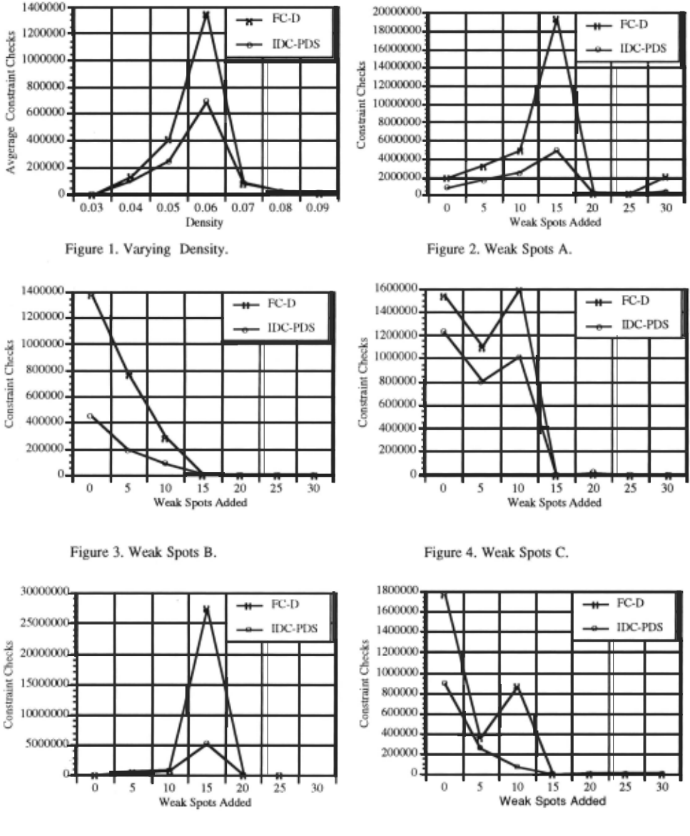
Figure 6. Weak Spots E.

6.3 Weak Spots

For each problem in the .06 set we processed problem variables to create a sequence of problems, introducing local "weak spots" into the original problem, either by removing or by weakening constraints. As we shall see, such local weak spots can be present in problems of extreme overall difficulty. Indeed, to a degree, it appears that local weak spots can actually increase overall problem difficulty. For forward checking, we might expect this, as forward checking around weakly constrained values produces relatively little pruning.

Figure 2 plots constraint checks for problems in one of these sequences. The flrst problem represented is one of the original .06 problems. We added weak spots to this problem, one at a time, by repeatedly picking a variable V, at random, that was involved in more than three constraints, and then randomly removing constraints involving V until only three remained. Each problem in Figure 2, after the ftrst, includes ftve more weak spots.

We observe a "complexity peak" induced, interestingly enough, by added weak spots. And we observe that IDC­ PDS dramatically "flattens" the complexity peak. IDC-PDS does very well both on the hardest problem that has no solution (15 weak spots added) and on the hardest problem that does have solutions (30 weak spots added).

IDC-PDS does have more overhead than FC-D, but IDC­ PDS can achieve a significant advantage in cpu time as well. In this sequence IDC-PDS has better cpu time on four of the seven problems, including the most difficult one: 12,162 seconds to 20,831 seconds. Bear in mind also that we are conducting constraint checks here by consulting efficiently hash-coded tables. In a real problem constraint checks could require significant calculation,. which is one reason they are a significant measure of CSP algorithm performance. Finally, observe that we are not trading constraint checks for some other form of table lookup, as can occur in "memory-based" algorithms.

Figures 3 through 6 shows the constraint check results for similarly induced problem sequences starting with the other four problems in the .06 set. Four of the five sequences exhibit a weakness-induced complexity peak, where IDC-PDS performance excels (though in two problems effort initially decreases). In one of these problems IDC-PDS completely eliminates the peak present in the FC-D results. In that sequence IDC-PDS achieves a full order of magnitude improvement over FC-D (70,528 constraint checks to 870,307 constraint checks) on a problem with solutions. The ftfth sequence, the only one where even the original problem has solutions, exhibits no significant weakness-induced peak; however, IDC-PDS superiority is still manifest. (Note that the scale on the constraint checks axis differs in the four graphs.)

In Figure 5 the effort for the last problem in the sequence is not plotted. FC-D tested at close to 5 million constraint checks while IDC-PDS with an IDC choice factor of 1.5

tested at close to 50 million constraint checks. However, again adding the inconsistency count value ordering heuristic made a dramatic difference: FC-D and IDC-PDS both required only 7,773 checks, all but 797 of them for computing the inconsistency counts! This problem does have solutions. Adding the value ordering for the problem at the plotted peak in this sequence (15 weak spots added), where there are no solutions, has a relatively small effect, as one might expect. (The value ordering does not always trivialize problems with solutions. The last problem in the sequence in Figure 2 becomes much simpler with the value ordering, but still requires almost 100,000 constraint checks with FC-D, and about half that with IDC-PDS.)

We also conducted a few experiments where weak spots were added by loosening rather than removing constraints, changing the local tightness rather than the local density. Problem sequences were generated where each successive problem contained flve more weak spots, generated in this new way, choosing variables randomly for creating weak spots. To create a weak spot at a variable all the constraints involving the variable had consistent pairs, chosen at random, added as needed for the tightness of each constraint times the degree of the variable to be less than one. (If this required adding all possible pairs to a constraint, the weakening was not carried out. If none of the constraints needed and permitted weakening, another variable was chosen at random to work on instead.)

We observed a complexity peak pattern similar to the one induced by removing constraints. For a sequence beginning with the original problem used in Figure 2, but inducing weak spots in this alternative manner, the peak occured at 10 added weak spots and went up to close to 50 million constraint checks for FC-D, but only about 10 million for IDC-PDS.

One might expect that many realistic problems will be inhomogeneous enough to contain some weak spots. Ironically, it appears that local weakness can dramatically increase overall problem difficulty. Thus a technique, like IDC decomposition, that is able to exploit weaknesses in hard problems seems highly desirable.