Numerical Interval Simulation: Combined Qualitative and Quantitative Simulation to Bound Behaviors of Non-Monotonic Systems

1 Introduction

Mathematical models of complex physical systems cannot be precisely defined in many cases, either due to lack of knowledge or because parameters and functions change over time according to unknown phenomena. Nevertheless, it is often possible to provide reasonable bounds for the parameters and functions. Bounds on parameters are interval ranges. Bounds on incompletely known functions take the form of a pair of functions, one to provide an upper bound and another to provide a lower bound. Such models that can integrate qualitative and quantitative knowledge are called semi-quantitative models. They can represent important classes of complex systems such as chemical, electro­ mechanical, nuclear, thermal, steel and other industrial processes [Vescovi et al., 1993].

Many qualitative simulation methods are based on constraint propagation. They generate all possible states and use filtering techniques to eliminate impossible ones. Semi-quantitative methods such as Q2 [Kuipers and Berleant, 1988] and Fu-Sim [Shen and Leitch, 1990] add numerical information and take advantage of it in the filtering process. The basic algorithm remains the same.

* This research is in part supported by the Advanced Research Projects Agency, ARPA Order 8607, monitored by NASA Ames Research Center under grant NAG 2-581, and by NASA Ames Research Center under grant NCC 2-537.

Such semi-quantitative methods do not fully exploit the quantitative knowledge and produce only weak predictions across time intervals. This is primarily due to the limitations of interval propagation across derivative constraints. The mean value theorem is used to constrain the ranges of a variable at two adjacent time points tn and tn+ 1, where tn and tn+ 1 are the temporal boundaries of a qualitative state. Those methods do not reason about the behavior of the system within a qualitative state.

This paper presents Numerical Interval Simulation (NIS), a complete method that produces more precise simulations of semi-quantitative models. NIS is complete in the sense that its solutions bound all the solutions of the semi­ quantitative model. NIS performs numerical simulations using maximal and minimal values for the derivatives of the state variables. In order to calculate such maximal and minimal values, NIS uses interval arithmetic to calculate intervals containing the possible values of the derivatives and takes their maximum or minimum respectively. The method replaces the use of the mean value theorem with explicit integration. NIS also produces tighter predictions than interval simulators as defined in [Moore,1979].

NIS was presented at the 1992 Qualitative Reasoning workshop [Vescovi and Trave-Massuyes, 1992]. At that same workshop, Kay and Kuipers also presented their work on dynamic envelopes. Both techniques share the same fundamental insights. Subsequent development has lead in different directions, although it should be possible to unify the two lines of work. NIS has been extended to handle non-monotonic functions and forcing functions, whereas the dynamic envelope method is more closely integrated with the QSIM [Kuipers, 1986] formalism. The dynamic envelope method of Kay and Kuipers [1993] derives and numerically simulates "extremal systems" composed of "extremal equations" that are bounds on the derivatives of the state variables. Such "extremal systems" have been automatically generated only for systems of monotonic functions.

NIS is an extension of the fuzzy simulation methods for linear systems proposed in [Vescovi, 1991] and [Vescovi and Trave-Massuyes, 1992]. We claim that the extension presented in this paper to handle nonmonotonic functions and forcing functions is fundamental to simulate real-world nonlinear complex systems. We demonstrate the usefulness of NIS by presenting its successful application to simulate a complex sintering process at CST Tubarao, a Brazilian­ Japanese steel company located in Brazil.

This paper is organized as follows: We first describe the Numerical Interval Simulation method. Second, we show two examples of numerical interval simulation of systems of ordinary differential equations composed of nonmonotonic functions. The first system represents an electrical system with power supplied by an AC generator, and the second represents an inverted pendulum attached to an electric motor. We then discuss the mathematical properties of the method. We finally present the application of NIS to a complex industrial process. We close with a discussion of related work and conclusions.

2 Numerical Interval Simulation

The Numerical Interval Simulation method takes as input a semi-quantitative model and generates upper and lower bounds on the trajectories of each of the state variables in the model. ·

The semi-quantitative model is composed of a set of equations, interval bounds on the constant parameters used in the equations, and interval bounds on the initial values of the state variables. The equations are (non-) linear first-order ordinary differential equations (ODEs) of the form:

The functions fk can contain the standard arithmetic operators such as addition, subtraction, multiplication, division, exponential, logarithm, sines, cosines, and constant parameters. In addition, fk can also contain intervals in place of constant parameters and interval functions that bound the values of the actual parameters and functions. Interval functions are functions that take intervals as arguments and return an interval. In other words, fk can contain, instead of a real-valued function g(t, XJ, ... xn). an interval function h(t, i], ... in) such that g(t, x], ... xn) E h(t, i], ... in) where ij's are intervals and Xj E ij for j = I to n.

NIS performs numerical simulation, using extremal values for the derivatives of the state variables. Such extremal values for the derivatives are calculated in the following manner:

• First, NIS uses interval arithmetic to calculate the interval of possible values for the derivatives of the state variables [Moore, 1979]. Since the functions fk can contain intervals (as parameters) and interval functions, the arithmetic operators in fk are actually their corresponding interval arithmetic operators, andfk are interval functions as well. NIS uses fk to calculate the intervals for the values of the derivatives.
• Second, NIS takes the maximum or minimum of the resulting interval, depending on whether the maximal or minimal derivative is required.

Later in the paper, we show that NIS is complete in the sense that its result is guaranteed to bound all the possible solutions of the semi-quantitative model. The only restriction for the functions fk is that they must be continuous over the intervals considered in the simulation. It means that functions fk can be composed not only of monotonic functions but also of nonmonotonic ones. NIS allows nonmonotonic functions over the reals such as multiplication, sine, cosine, exponential and logarithm, and the arbitrary interval functions can also bound a set of nonmonotonic arbitrary real functions.

The NIS method calculates maximal and minimal values for the derivatives at a given instant tn. Such extremal values are used by a numerical simulator to determine the value of the state variables at the next instant tn+ J. Several different methods could be used to perform the numerical simulation. We present below NIS using both the Euler's method and the Runge-Kutta method.

2.1 Euler's Method NIS

Let Xk(t) = [Xkmin(t), Xkmax(t)] be the interval such that its lower and upper bounds correspond to the minimum value Xkmin(t) and the maximum value Xkmax(t) of state variable Xk at timet respectively. In the remainder of this paper, we will use the notation [b) for the point interval {b, b) for brevity. The Euler's method NIS for each simulation step can be described as:

1. Calculate the maximum omax(tn)i and the minimum Omin(tn)i values for the derivatives of State variables Xi at instant tm in the following manner:

where

Notice that, the functions fi are calculated taking as arguments the real maximal value Ximax(tm) and the real minimal value Ximin(tm) of state variables Xi at instant tm respectively, instead of using the interval [Ximin(tm). Ximax(tm)J. This is fundamental to provide accurate simulations and will be discussed in more detail later in the paper.

1. Calculate the maximum bound Ximax(tm+ J) and minimum bound Ximin(tm+ J) at instant 1m+ J with the given step size of 8t:

2.2 Runge-Kutta NIS

We presented the Euler's method in two steps by first calculating the extremal values for the derivatives and second by caiculating the values of the state variables for aims of clarity. With the Runge-Kutta NIS, the extremal values for derivatives are calculated several times inside each iteration of the method. We present below the four-stage Runge- Kutta NIS method.We use the symbols E9 and® to represent the interval arithmetic relations addition and multiplication respectively. The equations are given for the upper bound, Ximax· The equations for the lower bound are identical with min substituted for max throughout.

ki1max = Ot max(fi(tm. X1, X2···· [XimaxJ. .. Xn)) ,

1 1 ki2max = 8t max(fi(tm + 28t, XJ 1$ [2] ® fk11min,

1 1 kj Jmaxl · ... , [Ximax + 2kilmaxl · ... , Xn 1$ {2] ® fknJmin, knJmaxl))

1 1 ki3max = 8t maxifi(tm + 28t), XJ 1$ {2] ® [kJ2min,

ki4max = 8t maxifi(tm + Ot, xjl${kJ3min, kJ3maxl · ... , [Ximax + ki3maxl · ... , xnl$fkn3min, kn3maxm·

2.3 Two Examples

In this section, we show NIS simulations of two electro­ mechanical systems. Each physical system is represented by ODEs that include.nonmonotonic functions.

Coupled two-stage electrical system

The first system is the coupled two-stage electrical system shown in Figure 1. The first stage is an RL series circuit with input DC voltage Vin provided by a battery. The second stage is an RC parallel circuit with input current lin provided by an AC generator. The current lin is a sinusoidal signal with amplitude and frequency directly dependent on the first stage circuit output current fL.

The following second-order system represents an instance of a such device:

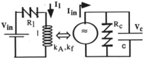
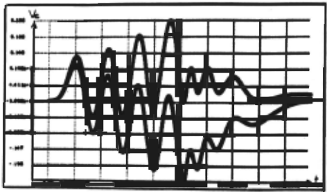
Figure 2 shows a NIS simulation of such system, given the following parameter and initial values:

Rt = [408, 410] mD,

l = 2 H, Rc= [400, 500] K.Q, c = 10 j.JF, kA = £16, 18110-8, kJ= f/23, 1251 10-1. It(O) = 0 A, and Vc(O) = 0 V.

Inverted pendulum

The second example is a well known problem in nonlinear mechanics, known as the inverted pendulum. The pendulum is a stiff bar of length L which is supported at one end by a frictionless pin. The support pin is given a rapid up-and· down motion s by means of an electric motor, s = A sin (JX. Application of Newton's second law of motion yields the equation L 0"=( g - co2 A sin co()) sin (), where () is the angular position of the bar (0 = 0 when the bar is directly above the pin), and g is the acceleration due to gravity.

Following is the second-order system representing the inverted pendulum:

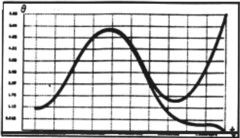
Figure 3 shows a NIS simulation of such system, given the following parameter and initial variables values:

g = 386.09 inlsec2, L = 10 in, A = [0.5, 0.55] in, a>= [5.3, 5.4] radlsec, 1C 9(0) = 3 rad, and 86(0) = 0 radlsec.

2.4 Properties of NIS

We have analyzed some computational properties of NIS, namely completeness and soundness. NIS can be shown to be complete, but not sound.

About Completeness

NIS is complete in the sense that its result is guaranteed to bound all the possible solutions of the semi-quantitative model. The proof of completeness, which is provided in details in [Vescovi et al., 1995], basically follows the steps below:

• Consider the semi-quantitative model x'k = fk(t, XJ, x2 · ... xn). where xk(to) E Iok fork= J, ... n.
• The function fkmax = (maxifk(t, XJ, ... [xkmaxl · ... Xn)) + E), E > 0, E ~ 0, calculated by NIS is such that :
• 'rft, Xkmax E R, 'rfxi, X2, ... Xn E /, 'rfx'k E R I X'k E fk(t, Xi, ... {XmaxJ · ... Xn), x'k < fkmax(t, Xi, ... [Xkmaxl · ... xn). 1

1 The value £ is actually considered negligible by the "'iS simulation method.

This is straightforward to prove since NIS uses inte~val arithmetic operations that calculate the set of all poss1~le values for the functions fk and only then takes Its maximum.

• For Xkmax such that x'kmax = fkmax(t, Xi, X2···· Xkmax · ... xn). we can prove that 'rft Xk(t) ~ Xkmax(t). The proof is based on the fact that, since the functions fk are continuous and Xk(tO) 5 Xkmax(tO). Xk has to be equal to Xkmax first in order to become greater than Xkmax . Since at any crossing point the derivative of Xkmax is greater than the derivative of Xk, Xk will be only smaller or equal to Xkmax at an arbitrarily small time after the crossing point and Xk does not become greater than Xkmax·
• In a similar manner, considering another function fkmin· we prove that 'rf t, Xkmin(t) ~ Xk(t).

About Soundness

Soundness is the property of predicting behaviors that are solution of at least one instance on the semi-quantitative model. Although NIS is not sound in general, the method is very precise in most cases. In this section we first discuss why NIS is usually precise by comparing the method to our first approach for interval simulation [Vescovi, 1991]. We then discuss and show a particular case in which the method diverges after a couple of interactions.

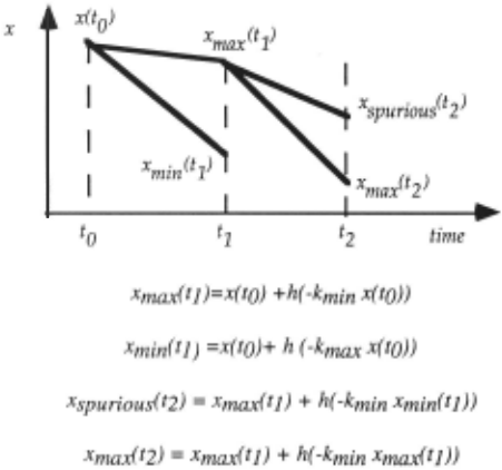
In order to point out why spurious behaviors are produced, we will recall our first approach for interval simulation [Vescovi, 1991]. The idea with the former method was to extend a numerical method by substituting its operators by the interval arithmetic correspondents. The extended method is complete but produces too much spurious values. The main reason is that the arithmetic interval operations are applied without taking into account the interaction among variables. Consider the first order system x' = -kx, there is a strong relation between x and x', and both variables are operands in the extended Euler's method:

x(tn+i) =x(tn) $(h ®x'(tn)) x(tn+i)= x(tn) $(h ®(B(k ®x(tnJ))

The possible values for x(tn+ i) are only those calculated considering unique values for x(tn) in eq.2. The extended method, however, combines all the possible values for x(tn) and x'(tn). Imagine xi, x2 such that xi, x2 E x(tn). the method considers the combination x(tn) =xi, and x'(tn) calculated for x(tn) = x2, which would probably produce a spurious value for x(tn + i ). Interactivity is partially overcome by NiS, since the functions fi take only the maximum Ximax(tn) or minimum Ximin(tn) of state variable x;. instead of the full interval fximinOn). Ximax(tn)]. For example, the NIS Euler's method of the first order system x'=-ks, with k= fkmir~> kmaxl. is

We can easily prove that the interval [Xmin (tn+1), Xmax (tn+ 1 )] produced by N1S is always a sub-interval of x (tn+ 1) produced by the extended method. Figure 4 illustrates this. The value Xspurious(t2), calculated by the extended method, would surely be a spurious value greater than xmax(t2), calculated by N1S.

The interval simulation showed in Figure 2 is a very precise simulation. The interval shrinks towards the end of the prediction of an oscillatory behavior, what would not be the case with most semi-quantitative methods, specially interval simulators.

However, other cases of interactivity between the state variable and their derivatives can occur. For example, with systems of the form

the interactivity is among Xi and other variables appearing in the equation of x'i· NIS simulations of such systems tend to become unstable after several iterations. The inverted pendulum and other oscillatory systems are of this type. Figure 3 illustrates such an instability.

3. The Complex Sintering Process

In this section, we present the successful application of NIS to predict behavior of a complex sintering process at CST Companhia Siderurgica de Tubarao, a steel company located in Brazil. The sintering process continuously produces sinter ore with various kinds of fine iron ore as the raw material and lime stone as the binder. The process has two major goals: One is the stabilization of operation to produce strong sinter ore of uniform size as the ferrous burden of the blast furnace. Another is optimization of the process to minimize the production cost under various conditions and processing throughout the whole iron works. Figure 5 illustrates the sintering plant. The granulated raw material in the surge hopper is fed across the sinter bed width and is ignited by the furnace. The material burns from the surface toward the bottom by the downward air flow through the wind boxes. The material is shifted by the sinter bed towards the cooler.

The goal of the process operator is to control the sinter bed speed in order to maximize productivity while maintaining safety. Too low a speed causes low sinter production and quality; high speed causes burning material to fall into the cooler, damaging the equipment and possibly causing a fire. An observable variable called the burn through point, Btp, is the primary variable to control. The Btp is supposed to be maintained between 65 and 78%. Btp below the lower boundary corresponds to low sinter quality condition and lost productivity, while Btp above the higher boundary corresponds to a dangerous operation condition. The ideal is to keep the Btp in between 70 and 75%.

Raw Material f

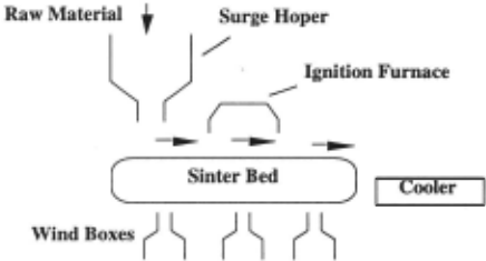
A precise model of the sintering process is not available due to the complexity and experimental nature of the process. Indeed, the relations among variables change during the operation, influenced by unknown phenomena. For example, the coefficients significantly change whenever there is a significant change in the quality of the raw material; this is very difficult to monitor. However, it is possible to define boundaries for the relations and parameters. Included in the semi-quantitative model of the sintering process used by NIS is the first order relation (the NIS simulated model actually contains a dozen of these first­ order relations), Btp' = P 106( t - -r) - g( Btp ); where 'f is the constant delay between Btp and pressure P 106, and g is a piece-wise linear function. Figure 6 shows the given boundaries for g(Btp). For more details, see [Vescovi et al., 1993].

Actual productivity, safety and reliability requirements demand optimum operation. In the case of the sintering process, Btp is to be kept as close as possible to 75%. Small deviations can have significant effects on the process. A Btp increase of around 3% when its value is at 75% correspond to a very dangerous operation region that can cause fire and damage to the coolers. Predictions that are too wide, either due to lack of knowledge, or weaknesses in the simulation method, are simply useless. Many hours of operation during different periods of the year were simulated, and the results obtained by NIS were very successful. With rare exceptions, the actual behavior of the process was always bounded by NIS simulations (the rare exceptions ocurred because of modeling errors as opposed to NIS errors). Furthermore, the predictions were considered tight enough to be useful.

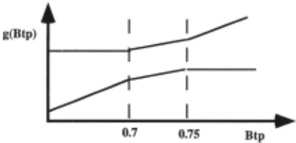
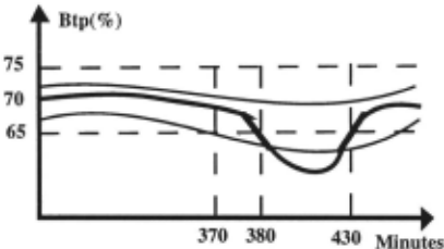
Figure 7 shows an example of a NIS predicted behavior (the two outer thin lines) and the observed behavior (the thick line) of the Btp. The NIS simulation failed in the interval [380, 430] minutes, indicating that the boundaries were not well chosen in this operating region. This is not of great concern since the system is not supposed to operate in this region (Btp smaller than 65%). This undesirable behavior occurred in reality because of an operator mistake. Notice that the NIS simulation predicted that the Btp would penetrate the region below 65% at time 370 minutes. An on-line monitoring system would have thus advised the operator about such possibility, and it could have been avoided.

4. Related Work

Research in different areas such as qualitative physics, sensitivity analysis, tolerance banding and interval analysis address the problem of combining qualitative and quantitative knowledge. We will first discuss the methods outside qualitative physics.

Sensitivity analysis [Deif, 1986] is used to predict the effect of small-scale perturbations to a system. Tolerance banding [Lunze, 1989] is used to predict large-scale uncertainties. Both methods are normally restricted to linear models and allow uncertainties of parameters and initial values only.

Interval Analysis Simulators [Moore, 1979; Markov and Angelov, 1986] are close related to NIS, in which they also simulate semi-quantitative differential equations by recasting numerical simulators to work with interval arithmetic. However, both NIS and the dynamic envelope method produce tighter simulations than the mentioned interval simulators (see [Kay, 1995] for more details). Basically, the method described in [Moore, 1979] consists in iteratively calculating the intervals Ai = X(tk) + [0, h) * F(Ai-1 ), given X( tO) and Ao which is a bound on X over the interval [tk, tk + h). Inclusion monotonicity garantees that the Ai intervals always shrink. The intervals Ai, which are bounds for the variables X, are the arguments for the derivative interval function F. The function F calculates intervals much larger than those calculated by NIS, which passes only fximaxl or [Ximinl as arguments for the derivative functions instead of the entire interval [Ximin. Ximaxl , as discussed in section 2.4. Such interval simulators do not take into account the interactivity among the variables. By analysing the method of calculating Ai, we can see that the prediction uncertainty will always increase with increasing time. It would thus be impossible with such a method to obtain precise results as those showed in figure 2 where the interval shrinks towards the end of the prediction of an oscillatory behavior.

Inside the scope of qualitative physics, the first semi­ quantitative methods such as Q2 [Kuipers and Berleant, 1988] and Fu-Sim [Shen and Leitch, 1990] do not fully exploit the quantitative knowledge available in the semi­ quantitative model and produce only weak predictions across time intervals. As model precision increases, NIS produces more precise simulations than Q2 or Fu-Sim. The method replaces the use of the mean value theorem with explicit integration over time.

To establish the temporal correspondence between the observed values and the predictions, the sintering application uses synchronized sampling as most industrial process monitoring systems do. Tracking the process is thus significantly facilitated. The imprecision of the semi­ quantitative model only affects variable values estimates. That provides a firmer ground for comparing the results of the simulation with real observations, which is crucial in real time monitoring systems. In semi-quantitative methods like Q2 or Fu-Sim, temporal durations are calculated with the first order Taylor-Lagrange formulae using quantity space values in the form of numeric or fuzzy intervals. It was shown in [Missier, 1991] that the first order Taylor­ Lagrange formulae is scarcely sufficient to provide significant information. This is true, independent of the weakness directly related to a weak quantity space, at the neighborhood of critical points for which the derivative reaches zero. Indeed, zero derivative leads to one infinite boundary for the duration estimate. As a result, time durations calculated for adjacent states are often widely overlapped. It may happen that a given time instant belongs to several consecutive states, implying that variable values at this instant are very weakly constrained.

Most closely related to NIS is the dynamic envelope method [Kay and Kuipers, 1993]. Both methods numerically simulate extremal systems. NIS uses interval arithemetic to calculate the extremal values for derivatives at each simulation step, whereas the dynamic envelope method generates the extremal systems a priori. The dynamic envelope method inherits certain limitations from the QSIM formalism upon which it is built. First, it does not allow forcing functions such as A sin co-r in the example in Section 2.3 . Forcing functions cannot be reasonably specified in a purely qualitative framework, because the events generated by the forcing function must be exhaustively interleaved with the normal qualitative events. This results in a combinatoric explosion. Second, the QSIM formalism does not allow for non-monotonic function in equations other than multiplication. The dynamic envelope method also benefits from the qualitative representation. QSIM is able to split divergent behaviors, which allows the dynamic envelope method to provide separate, tighter, bounds on each qualitative behavior, rather than a single, broad, bound that covers all of the behaviors.

NIS can simulate systems involving nonmonotonic functions and allows use of forcing functions. Since a large class of complex industrial processes are modeled by nonmonotonic functions and include force functions, the capability of handling such functions constitutes an important contribution to the field of qualitative physics.

NIS simulations of certain oscillatory systems can be unstable. The same limitation occurs with the dynamic envelope method. An alternative, which consists in intersecting the results of the dynamic envelope method and of Q2, was proposed in [Kay and Kuipers, 1993] in order to improve the results of the simulation in such cases. We are considering the integration of NIS with the methods under development at the University of Texas.

5. Summary

The Numerical Interval Simulation method produces high precision simulations of semi-quantitative models. The method is complete in the sense that its solutions bound all the solutions of the semi-quantitative model. As the precision of the semi-quantitative model increases, the method produces more precise simulations than former semi­ quantitative methods like Q2 or Fu-Sim. Although NIS produces the same results as the dynamic envelope method when simulating systems involving only monotonic functions, the method also simulates systems containing arbitrary continuous, nonmonotonic functions. NIS also allows use of forcing functions. We claim that such level of generality is fundamental to simulate real-world nonlinear complex systems.

We demonstrated the usefulness of NIS by presenting its successful application to simulate a complex sintering process at Companhia Siderurgica de Tubarao, a Brazilian­ Japanese steel company located in Brazil. The result shows that NIS is adequate to represent the available information and produces simulations with the required level of precision. The prototype has been tested and we are working to run NIS on-line as an adviser to the sintering process operators.

Acknowledgments

We would like to thank Marcelo Lame go and Cristiano Dalvi for their work in modeling the CST sintering process.