
Scaling up Self-Explanatory Simulators: Polynomial-time Compilation
Proceedings of the Fourteenth International Joint Conference on Artificial Intelligence. Qualitative Reasoning and Diagnosis. Pages 1798-1804.
© 1995 International Joint Conferences on Artificial Intelligence
Abstract
Self-explanatory simulators have many potential applications, including supporting engineering activities, intelligent tutoring systems, and computer-based training systems. To fully realize this potential requires improving the technology to efficiently generate highly optimized simulators. This paper describes an algorithm for compiling selfexplanatory simulators that operates in polynomial time. It is capable of constructing self-explanatory simulators with thousands of parameters, which is an order of magnitude more complex than any previous technique. The algorithm is fully implemented, and we show evidence that suggests its performance is quadratic in the size of the system being simulated. We also analyze the tradeoffs between compilers and interpreters for self-explanatory simulation in terms of application-imposed constraints, and discuss plans for applications.
- Forbus, K. and Falkenhainer, B. Self-explanatory simula- tions: An integration of qualitative and quantitative knowledge, Proceedings of AAAI-90.
- Forbus, K . and Falkenhainer, B. Self-Explanatory Simu- lations: Scaling up to large models, Proceedings of AAAI- 92.
- Iwasaki, Y. & Low, C. Model generation and simulation of device behavior with continuous and discrete changes. Intelligent Systems Engineering, 1(2), 1993.
- Amador, F., Finkelstein, A. and Weld, D. Real-time self- explanatory simulation. Proceedings of AAAI-93.
- Forbus, K. Towards Tutor Compilers: Self-explanatory simulations as an enabling technology, Proceedings of the Third International Conference on the Learning Sciences, August, 1991.
- Neville, D., Notkin, D., Salesin, D., Salisbury, M., Sherman, J., Sun, Y., Weld, D. and Winkenbach, G. Electronic 'How Things Work' Articles: A Preliminary Report. IEEE Transactions on Knowledge and Data En- gineering, August 1993.
- Gautier, P. and Gruber, T. Generating explanations of device behavior using compositional modeling and causal ordering. Proceedings of AAAI-93.
- Forbus, K. Self-Explanatory Simulators: Making comput- ers partners in the modeling process. In Carrete, N. P. & Singh, M.G. (Eds.), Qualitative Reasoning and Decision Technologies, CIMNE, Barcelona, Spain, 1993.
- Forbus, K. and Whalley, P. (1994) Using qualitative physics to build articulate software for thermodynamics education. Proceedings of AAAI-94, Seattle.
- Sgouros, N. Integrating qualitative and numerical models in binary distillation column design, Proceedings of the 1992 AAAI Fall Symposium on Design of Physical Sys- tems, October, 1992.
- llAmador, F. 1994. Self-Explanatory Simulation for an Electronic Encyclopedia. Ph.D. dissertation, Department of Computer Science and Engineering, University of Washington.
- 12Forbus, K. The Qualitative Process Engine. In Weld, D. and de Kleer, J. (Eds.) Readings in qualitative reasoning about the physical systems, Morgan-Kaufmann, 1990, pp 220-235.
- 13de K1eer, J. An assumption-based truth maintenance system. Artificial Intelligence, 28(1986): 127--162.
- DeCoste, D. and Collins, J. CATMS: An ATMS which avoids label explosions. Proceedings of AAAJ91.
- Forbus, K. Qualitative Process theory. Artificial Intelli- gence,24, 1984 16
- Forbus, K. and de Kleer, J. Building Problem Solvers, MIT Press, 1993.
- Woods, E. The Hybrid Phenomena theory. In Proceed- ings of /JCAI-91, Sydney, Australia. IJCAI
- Forbus, K. Pushing the edge of the (QP) envelope. In Recent Progress in Qualitative Physics, Faltings, B. and Struss, P. (Eds.), MIT Press, 1992.
- Forbus, K. and Falkenhainer, B. Self-explanatory simula- tors. Manuscript in preparation.
- Roberts, B. and Forbus, K. The STEAMER mathemati- cal simulation. BBN Technical Report No. 4625, 1981.
- Forbus, K. and Gentner, D. Causal reasoning about quantities. Proceedings of the Eighth annual conference of the Cognitive Science Society, Amherst, Mass., August, 1986
- Skorstad, G. Finding stable causal interpretations of equations. In Faltings, B. and Struss, P. (Eds.), Recent advances in qualitative physics, MIT Press, 1992.
- Hollan, J., Hutchins, E., & Weitzman, L. STEAMER: An interactive inspectable simulation-based training system. AI Magazine, 5(2), 15-27.
References were extracted automatically from the PDF and may contain errors.
Full text extracted automatically from the PDF; figures, tables and equations may differ. The PDF is the version of record.
1. Introduction
Self-explanatory simulators [1,2,3,4] integrate qualitative and quantitative knowledge to produce both detailed de scriptions and causal explanations of a system's behavior. They have many potential applications in intelligent tutor ing systems and learning environments [5, 6] and engineer ing tasks [7,8]. One step towards realizing this potential is developing techniques that can operate efficiently on sys tems involving many hundreds of parameters, so that, for instance, complex training simulators can be generated automatically. This paper describes a polynomial-time method for compiling self-explanatory simulators and shows that it operates successfully on models larger than most industrial applications require. This paper considers only initial-value simulations of lumped-element (ordinary differential-algebraic) systems.
Section 2 reviews the basics of self-explanatory simula tors. Section 3 describes our new polynomial-time compi lation technique. Section 4 outlines the complexity analysis and Section 5 summarizes empirical results, including evi dence that its performance is quadratic in the size of the system bejng simulated. Section 6 identifies tradeoffs in constructing self-explanatory simulators in light of task re quirements. Section 7 outlines our plans for future work.
2. Self-Explanatory simulation: The basics
Traditional numerical simulators generate predictions of behavior via numerical computation using quantitative models of physical phenomena. Most simulators are written by hand, although an increasing number are generated by Brian Falkenhainer Modeling Research Technology Area Xerox Wilson Center MS 128-28E 800 Phillips Road, Webster, NY, 14580, USA
domain-specific toolkits. Modeling decisions, such as what phenomena are important to consider, how does the phe nomena work, how can it be modeled quantitatively, and how to implement the quantitative model for efficient com puter solution, are mostly made by hand. Domain-specific toolkits provide reasonable solutions to the last two prob lems, and with appropriate libraries they can simplify the first problem. However, the choices of how to translate the physical description into the conceptual entities supported by the toolkit, and which quantitative model to use from the library to model an entity, are still made by hand. Moreo ver, no existing toolkit provides the intuitive explanations used by scientists and engineers to describe how a system works. These intuitive, qualitative descriptions serve sev eral important purposes in building and working with simulations. First, they guide the formulation of quantita tive models by identifying what aspects of the physical situation are relevant. Second, qualitative descriptions are used to check the results of a simulation, to ensure that it "makes sense." Thus two advantages of self-explanatory simulation are increased automation and better explana tions [I].
Self-explanatory simulators harness the formalisms of qualitative physics to automate the process of creating simulators. Given an initial physical description, a qualita tive analysis of the situation reveals what conceptual entities are relevant to the task and what causal factors affect a pa rameter under different circumstances. This information is then used, in concert with quantitative information in the domain theory, to construct numerical simulation programs for the system. By incorporating explicit representations of conceptual entities (such as physical processes) in the simulator, causal explanations can be given for the simu lated behavior. Moreover, the qualitative representations allow automating some of the "reality checks" that an expert would apply in evaluating a simulation. For instance, a simulation of a fluid system which reported a negative amount of liquid in a container is not producing realistic results. This ability is called self-monitoring.
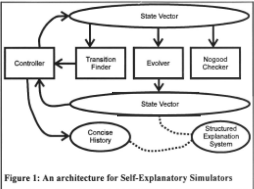
Figure I shows a typical architecture for self explanatory simulators. The state vectors are arrays of floating point and boolean values describing the state of the system at a particular point in time. The floating point val ues represent the values of continuous parameters, such as pressure and velocity. The boolean values represent the validity of statements about the physical system at that time, e.g., if liquid exists inside a container or if a particular physical process is acting. Given a state vector and a time increment, the evolver generates a state vector representing the state of the system after that time increment.
In many physical systems, the equations governing the temporal evolution of the system's behavior can themselves change, as when phase changes occur or flows start and stop. These changes occur at limit points, which mark the boundaries between qualitatively distinct behaviors. The transition finder (again see Figure I) detects the occurrence of limit points. The controller uses the transition finder and evolver to "roll back" the simulation to include all limit points in the simulated behavior. This increases the accu racy of the simulation because it ensures that the appropriate sets of equations are always used, and increases the accu racy of explanations because it ensures that causally impor tant events (e.g., reaching a phase transition) are included in the simulated behavior. The controller also is responsible for recording a concise history describing the system's qualitative behavior over time. This concise history is used in conjunction with a structured explanation system [9] to provide hypertext explanations of the system's behavior over time, including physical, causal, and mathematical descriptions. The nogood checker generates a warning if qualitative constraints are violated by a state vector, thus providing self-monitoring.
The first systems to generate self-explanatory simulators were compilers, doing all reasoning off-line to produce software that approached the speed of traditional simulators while providing causal explanations and self-monitoring. These compilation strategies were computationally expen sive. SIMGEN MK1 [1] used envisioning, an exponential technique, for its qualitative analysis procedure.
SIMGEN MK2 [2] exploited the observation that simu lation authors never explicitly identify even a single global qualitative state of the system being simulated, hence qualitative simulation is unnecessary for simulation con struction. Qualitative analysis is still necessary to deter mine what physical phenomena are relevant, for instance, but most exponential reasoning steps could be eliminated. SIMGEN Mk2 could construct simulators of systems larger than any envisioning-based system ever could (i.e., involv ing up to hundreds of parameters), such as a twenty stage distillation column [ 1 0). This advance in capabilities was not free: The tradeoff was that some explanatory capabili ties (i.e., efficient counterfactual reasoning) and self monitoring capabilities (i.e., the guarantee that every nu merical simulator state satisfied a legal qualitative state) were lost in moving from SIMGEN Mki to SIMGEN Mk2. As Section 3 explains, even SIMGEN Mk2 was subject to combinatorial explosions, because it was based on an A TMS. The techniques in this paper trade away more self monitoring to achieve polynomial-time performance.
An alternative to compiling self-explanatory simulators is to build interpreters that interleave model-building, model translation into executable code, and code execution [3,4). For example, PIKA [4] uses Mathematica and a causal ordering algorithm to decompose a set of equations into independent and dependent parameters and find an or der of computation. Every state transition which changes the set of applicable model fragments reinvokes this reason ing to produce a new simulator. ([ 1I] uses an incremental constraint system to minimize this cost.) One motivation for interpreters was the perceived slowness of compiler tech niques; by only building models for behaviors that are known to be relevant, presumably the overall time from formulation of the problem to the end of simulation would be reduced, even though the simulation time itself might be longer due to run-time reasoning. Such systems are not themselves immune from combinatorial explosions, and have never been tested on examples as large as compilers ( c.f. [I 0]), but on small examples interpreters can exhibit impressive performance.
It should be noted that the claim that PIKA is "5,000 times faster than SIMGEN MK2" [4] is problematic, for three reasons. First, the domain theories used by each sys tem were completely different. PIKA used just two model fragments, with built-in quantitative models containing ex ample-specific numerical constants. This is not realistic. By contrast, in keeping with the goal of increased automation, the domain models used in SIMGEN MK2 were similar to others used in qualitative physics, with quantitative infor mation added modularly. For instance, parameters such as fluid and thermal conductances and container sizes and shapes are explicit variables in our models that can be set by the simulation user at run-time. Second, the hardware and software environments used by the two systems were com pletely different, making the comparison figures meaning less. Finally, the factor of 5,000 claimed is based on one example only; the other example for which even roughly comparable data is available shows a difference smaller by a factor of I 0.
3. SIMGEN MK3: Compiling self-explanatory simulators in polynomial-time
We have developed a polynomial-time algorithm for compiling self-explanatory simulators. The improvements in complexity are purchased at the cost of reduced self monitoring and less compile-time error checking. However, the ability to quickly generate simulators for systems con taining thousands of parameters suggests that these costs are worth it. Here we outline the algorithm and explain how it works. We begin by describing why using an A TMS [ 16] was the source of exponential behavior in SIMGEN MK2. Next we examine the inference services needed to generate simulators, and show polynomial-time methods for achiev ing them. Finally, we outline the algorithm.
3.1 ATMS: The exponential within
A TMS' are often used in qualitative reasoning when many alternative situations are being explored [12]. A qualita tive state can be defined as a set of assumptions and their consequences, so that states (and partial states) can be con cisely represented by ATMS labels [13]. The labels in an A TMS database provide a simple and elegant inferential mechanism for simulation generation. For instance, the code needed to generate the truth of a proposition could be generated by interpreting the label as a disjunction of con junctions, with each assumption becoming a procedural test. (For instance, the boolean corresponding to a particular liquid flow occuring might be set to TRUE if the boolean corresponding to the fluid path being aligned was TRUE and the numerical value for the pressure in the source were greater than the numerical value for the pressure in the des tination.) Labels for causal relationships were used to infer what combinations of them could occur together, and hence what mathematical models were needed. (For instance, there can be several distinct models for flow rates, depending on whether or not one is considering conductances, but no two of these models can ever hold at the same time.) Using la bels made certain optimizations easy, such as proving that two distinct ordinal relationships were logically equivalent and thus allowing the same test to be used for each, which enhances reliability. (For example, in a spring-block oscilla tor the relationship between the length of the spring and its rest length determines the sign of the force.)
Unfortunately, even when we did not perform qualita tive simulation at all, the number of environments generated by the A TMS grew exponentially with the size of the sys tem modeled. Empirically, we found that the source of this growth was the transitivity inference system, whose job it is to infer new ordinal relationships via transitivity and mark as inconsistent combinations of ordinal relations that violate transitivity. This makes sense because dependency net works in which assumptions are justified by other assump tions, and especially those containing cycles, lead to expo nential label growth [14]. The majority of assumptions in a typical analysis are ordinal relations, and cyclic dependen cies are inherent in transitivity reasoning. Transitivity rea soning cannot be avoided when using an A TMS in simula tion generation, because without it the labels will include impossible combinations. We conclude that the ATMS must be abandoned to generate simulators in polynomial time.
3.2 How to get what you really need without exponential performance
What is the minimum reasoning needed to generate a simu lator for a physical scenario? (l) The model fragments of a domain theory must be instantiated to identify the relevant physical and conceptual entities and relationships (e.g., the existence of contained fluids and phase change processes). (2) The causal and quantitative relationships that follow from them must be determined, to generate the appropriate causal accounts and mathematical models (e.g., models that allow the level of a liquid to be computed given its mass, density, and specifications of its container). (3) The truth values of propositions corresponding to these relationships holding and/or entities existing (e.g. whether the liquid ex ists at a particular time, and if so, what processes are acting on it) must be inferred to control the operation of the quanti tative models. The performance of any compiler and the quality of the code it produces depends on how these ques tions are answered. For instance, if the shape of a container can be fixed at compile-time, then the model for liquid level depending on that shape can be "hard-wired," but if the shape is unknown, a run-time conditional must be inserted and code representing alternative models generated.
Three techniques provide the inferential services needed for polynomial-time simulation generation. (l) Reification of antecedents: When instantiating model fragments, create explicit assertions concerning their antecedents, in addition to installing the appropriate dependency network. One ex ample is
((liquid-flow (C-S water liquid f) Pl G) :ANTECEDENTS ( :AND (> (A (amount-of-in water liquid F)) ZERO) (aligned Pl) (> (A (pressure (C-S water liquid f)) (A (Pressure G)))))(The creation of such assertions is automatic, and is transparent to the domain modeler.) Such reified antece dents are also generated for causal relations and mathemati cal models. These antecedent assertions are used by the compiler in generating truth value tests for propositions. (2) Symbolic evaluation: If the truth value of a proposition is known at compile-time, it is presumed to hold universally. For instance, if a valve is known to be open at compile time, the simulator produced should always presume the valve is open, but otherwise the simulator should include explicit tests as to whether or not the valve is open and change its operation accordingly. A simple symbolic evaluator provides this information, using the reified ante cedents and a logic-based TMS [16]. Given a proposition, it returns TRUE, FALSE, or MAYBE, according to whether the proposition is universally true, universally false, or can vary at run-time. (3) Deferred error checking: Finding errors at compile-time can require exponential work. One example is proving that exactly one of the quantitative models for a specific phenomena must hold at any given simulated time. Such exponential inferences can be avoided by substituting run-time conditionals. For instance, if there are N mathematical models of a phenomena, insert a condi tional test that runs the appropriate model according to the simulator's current parameters, and signals an error if no model is appropriate. This reduces self-monitoring, in that fmding such problems at compile-time would be useful. However, this solution is common practice in building stan dard simulators when its behavior might enter a regime for which the author lacks a good mathematical model.
3.3 The SIMGEN MK3 Algorithm
The algorithm is outlined in Figure 2. It is very similar to SIMGEN MK2 (described in [2]), so here we focus on how the above techniques are used.
Step 1: Creation of the scenario model
As before, we assume domain theories are written in a compositional modeling language, using Qua~itative Process theory [ 15] for their qualitative aspects. Smce the cost of qualitative reasoning was the dominant cost in ~IM�EN MK 1 and MK2, the tradeoffs in this step are crucial. The source of efficiency in interpreters like PIKA [4] and DME [3] is that they appear to do no qualitative reasoning beyond instantiating model fragments directly corresponding to equations.
Step 1 uses a qualitative reasoner to instantiate model fragments and draw certain trivial conclusions (i.e., if A>B then -,A=B). No transitivity reasoning, influence resolu tion or limit analysis is attempted. We use TGIZMO, a pub licly available QP implementation [16] fo~ our qualitative reasoner. We modified it in two ways. First, the pattern directed rules that implement many QP operations were simplified, stripping out inferences not needed . by ~he compiler. Second, we implemented an.tecedent rei~catwn by modifying the modeling language ImplementatiOn to assert antecedents explicitly in the database as well as pro ducing L TMS clauses.
Step 2: Constructing the simulator's state
Here the results of qualitative analysis are harvested to specify the contents of state vectors, the concise history, and the explanation system. The numerical parameters are the quantities mentioned in the scenario mode~.. Boolean ~a rameters are introduced for relevant propositions: the exis tence of individuals (EXISTS) and quantities (QUANTITY), the status of processes and views (ACTIVE), and any gr?und propositions mentioned in their antecedents, recumv~ly (except ordinal relations, which are computed by comparm~ numerical values). Each boolean parameter has an associ ated antecedents statement, a necessary and sufficient condition for the truth of the corresponding proposition.
As noted above, any proposition known to be true in the scenario model is presumed to hold universally over any use of the simulator. The compiler does not generate simulator parameters for such propositions, although ~hey are still woven into the explanation system appropnately. Every proposition whose truth value is not known in the scen.ario yields a boolean parameter whose value must.be ascertamed at run-time. This technique allows the compiler to produce tighter code by exploiting domain constraints. ~d user hint~. The symbolic evaluator decides what propositions are static and simplifies antecedents containing them.
Step 3: Writing the simulator code
To achieve flexibility compositional modeling demands decomposing domain knowledge into small fragments. This can lead to long inference chains, which if proceduralized naively, would result in simulators containing red~nd~t boolean parameters and run-time testing. Step 3.1 srrnph fies inference chains in order to produce better code. We use two simplification techniques: (1)"Symbolic evaluation exploits compile-time knowledge to simplify .expressions and (2) A minimal set of boolean parameters IS fo~nd by dividing them into equivalence classes, based on their ante cedents. That is, if a proposition A depends only on B, and B in tum depends only on C, and C either has an empty ante cedent or an antecedent with more than one ground term,
- Create scenario model by instantiating model fragments from domain theory
- Analyze scenario model to define simulator state vector and constituents of concise history and structured explanation system. . .
- Extract physical and conceptual entities
- Defme boolean parameters for relevant propositions
- Define numerical parameters and relevant comparisons
- Extract influences to create causal ordering
- Write simulator code
- Simplify antecedents of boolean parameters
- Compute update orders
- For numerical parameters, use causal ordering
- For boolean parameters, use equivalences and dependencies
- Write evolver code
- Write transition finder code
- Write nogood checker code
- Write structured explanation system
Figure 2: The SIMGEN MK3 Algorithm
then A B and C would be in the same equivalence class, and C 'w~uld be its canonical member. Each equivalence class is represented in the simulation code by a single boo lean parameter, although all original propositions are re tained in the explanation system to maintain clarity.
In Step 3 .2, the state space assumption, common in en gineering and satisfied by QP models [17], guarantees we can always divide the set of parameters into dependent and independent parts, with the independent parameters being those which are directly influenced (or uninfluenced) and with the dependent parameters computed from them. To gain a similar guarantee for boolean parameters we stipulate that the domain theory is condition grounded [ 18], an as sumption satisfied by all domain theories we have .seen in practice. An independent boolean parameter mentiOns n~ other boolean parameters in its antecedents. It could be um versally true or false, or its value could be determined at run-time by ordinal relations (e.g., the existence of a con tained liquid depending on a non-zero amount of that sub stance in liquid form in the container) or by the simulation user's assumption (e.g., the state of a valve). A boolean parameter that is not independent is dependent. The logical dependencies between boolean parameters defme an . order ing relation that can be used as the order of computatiOn for them.
The overall structure of the code produced by the com piler in steps 3.3 through 3.5 is the same as in SIMGEN MK2. The only change in step 3.6 is taking into account the simplifications in the boolean parameters, which. is s~mple so we ignore it here. In evolvers, the effects of direct mflu ences are calculated first to estimate derivatives, the de pendent numerical parameters are then updated, followed by the boolean parameters. The main impact of restricted in ferencing in writing evolvers arises in selecting quantitative models for updating dependent numerical parameters. For instance, a domain theory may have two quantitative models for the level of liquid as a function of mass, depending on whether the container is cylindrical or rectangular. If the compiler knows the shape of the container (via symbolic evaluation) it can install the appropriate model, otherwise it must provide both models in the simulator and write a run time conditional. The compiler must also handle models in which the equations governing a quantity vary over time. In SIMGEN MK2 these cases were handled by using influence resolution to see what combinations of qualitative propor tionalities could co-occur, constructing appropriate quanti tative models for each combination or signaling a compile time error if the domain theory failed to include an appro priate quantitative model. In SIMGEN MK3 we instead re trieve all the quantitative models for a parameter not ruled out via symbolic evaluation and write code that selects the relevant model based on evaluating the models' antecedents in the current state vector. The evolver code includes a test for none of the known models being relevant, and generates a run-time error in such cases.
In generating transition finders, restricted inference can lead to moot run-time tests, corresponding to physically impossible transitions. However, symbolic evaluation catches most of them, and this is not a serious drawback because inequality tests are very cheap. Generating nogood checkers is simplified: Previous compilers generated code based on A TMS nogoods to detect impossible behaviors. Much effort was wasted filtering the nogoods, since the vast majority of them were transitivity violations, which are ir relevant when ordinal relations are computed from known numerical parameters. SIMGEN MK3 simply uses the sym bolic evaluation procedure to see what ordinal relations are known to be impossible and test for those.
4. Complexity Analysis
A detailed complexity analysis is beyond the scope of this paper (but see (19]); here we settle for proving that the algorithm is polynomial.
Step 1: The only exponential behavior in previous compil ers occurred in this step, so its complexity is crucial. The time complexity is the sum of the time to instantiate model fragments and the time to draw conclusions with them. The cost of instantiation can be decomposed into two factors: The cost of pattern matching, and the size of the description produced by the operation of the system's rules. The cost of pattern-matching is polynomial in the number of antece dents [16]. We assume that both the scenario model and the domain theory are fmite, and that the number of new enti ties introduced by the domain theory for any scenario model is a polynomial function of the size of the scenario model. Domain theories with exponential, or even unbounded, creativity are possible in theory [18), but never appear in practice.
The number of clauses instantiated about any particular statement is bounded by a polynomial, since it is a function of (a) the number of relevant domain theory statements, which is always small and certainly independent of the size of the scenario and (b) the number of entities introduced is polynomial. Since the work of instantiation is the product of the number of instantiations and the work to perform each, the instantiation process is polynomial-time. Fur thermore, the dependency network so created is polynomial in size, as a function of the size of the domain theory and scenario model. This means that the cost of inference re mains polynomial in these factors, since we use an L TMS, for which the cost of inference is worst-case linear in the size of the dependency network (16]. we thus conclude that the time and space complexity of this step is polyno mial.
| Example | Mk2 | Mk3 |
|---|---|---|
| Two containers | 22.8 | 6.42 |
| Boiling water | 25.2 | 5.32 |
| Spring/Block | 6.4 | 1.85 |
| 3x3 container grid | 16286 | 54 |
Step 2: Most of the work in this step consists of fetching information from the TGIZMO database and constructing corresponding internal compiler datastructures, which is obviously polynomial time. The only other potentially expensive part of this computation is the symbolic evalua tion procedure. Symbolic evaluation of a ground tenn is performed by checking its L TMS label, which is constant time. Symbolic evaluation of a compound expression is a recursive analysis of the structure of the expression, ending in ground terms. The size of expressions is determined by the antecedents in the domain theory, and thus for any do main model a maximum size can be found for such expres sions independent of the size of the scenario model. Ergo symbolic evaluation is also polynomial in the size of the scenario model.
Step 3: Each of these computations involves simple polynomial-time operations (see [2]), the most expensive being sorting the numerical parameters via the causal order ing, sorting the boolean parameters via logical dependen cies, and computing the equivalence classes for boolean parameters. All of these are simple polynomial-time opera tions, operating over datastructures whose size is polyno mial in the initial scenario description, so they are polyno mial time as well.
| Grid Size | # quantities | # boo leans | # propositions | Compile time (sec) |
|---|---|---|---|---|
| 2 | 83 | 24 | 456 | 6 |
| 3 | 198 | 63 | 1131 | 19 |
| 4 | 363 | 120 | 2108 | 49 |
| 5 | 578 | 195 | 3387 | 105 |
| 6 | 843 | 288 | 4968 | 202 |
| 7 | 958 | 399 | 6851 | 356 |
| 8 | 1523 | 528 | 9036 | 586 |
| 9 | 1938 | 675 | 11523 | 927 |
| 10 | 2403 | 840 | 14312 | 1429 |
5. Empirical Results
SIMGEN MK3 is fully implemented, and has been tested successfully on the suite of examples described in [2]. In all cases it is substantially faster than SIMGEN MK2, as Table I shows. The simulators it produces, like those of SIMGEN MK2, operate at basically the speed of a traditional numeri cal simulator, with the only extra run-time overhead being the maintenance of a concise history for explanation gen eration. Currently the compiler's output is Common Lisp without any numerical declarations, and even with this per formance handicap, the simulators it produces run quite well on even small machines (i.e., Macintosh Powerbooks).
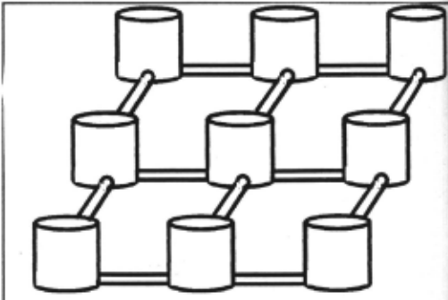
To empirically demonstrate that SIMGEN MK3's per formance is polynomial time, we generated a set of test ex amples similar to those used in [2]. That is, a scenario de scription of size n consists of an n by n grid of containers, connected in Manhattan fashion by fluid paths. Figure 3 illustrates for the three by three case. We generated a se quence of scenario descriptions, with n ranging from 2 to 10. (The reason we chose 10 as an upper bound is that the simulator which results contains just over 2,400 parameters, which is roughly three times the size of the STEAMER en gine room numerical model [20].) Extending the domain theory in [16], contained liquids include mass, volume, level, pressure, internal energy, and temperature as dynami cal parameters, as well as other static parameters (e.g., boiling temperature, specific heat, density). Containers can be either cylindrical or rectangular, with appropriate nu merical dimensions in each case. The liquid flow process affects both mass and internal energy. We then ran the compiler to produce simulators for each scenario, to see how its performance scaled. The results are show in Table 2. In an n x n grid scenario, there are n 2 containers and 2[n 2 -nJ fluid paths, so the numbers of parts in these exam ples ranges from 8 to 280. The count for quantities includes both static and dynamic parameters, and the count for boo leans includes both conditions controllable by the user (e.g., the state of valves) and qualitative state parameters, such as whether or not a particular physical process is occurring. The proposition count is the number of statements in the simulator's explanation system.
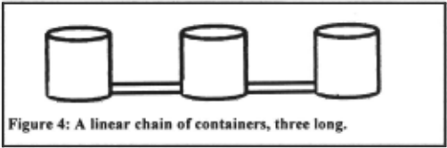
The theoretical analysis in previous sections suggests that the compile time should be polynomial in the number of parts in the system. A least-squares analysis indicates that this is correct: A quadratic model (O.Ol7r + 0.399P + 4.586, where P is the number of containers and paths) fits this data nicely, with X 2 = 0.03. Additional evidence for quadratic performance is found in Table 3, which shows the compiler's performance on examples constructed out of linear chains of containers. A chain of length N has 2N-J parts, i.e., N containers and N-1 fluid paths. Figure 4 illus trates. A least-squares analysis indicates again that a quad ratic model (O.OJ8r + 0.554P + 0.228, where P is the number of containers and paths) fits this data well, with X 2 = 0.004.
6. Tradeoffs in Self-Explanatory Simulators: Compilers versus Interpreters
Different applications entail different tradeoffs: Some po tential users have powerful workstations and can afford the best commercial software (e.g., many engineering organi zations), and some potential users have only hand-me-down computers and publicly available software (e.g., most US schools). Here we examine tradeoffs in self-explanatory simulation methods with respect to potential applications.
| N # quantities | # booleans | # propositions | Compile Time (sec) | |
|---|---|---|---|---|
| 2 | 38 | 9 | 194 | 2.05 |
| 3 | 58 | 15 | 305 | 3.43 |
| 4 | 78 | 21 | 416 | 5.02 |
| 5 | 98 | 27 | 527 | 6.66 |
| 6 | 118 | 33 | 638 | 8.72 |
| 7 | 138 | 39 | 749 | 10.5 |
| 8 | 158 | 45 | 860 | 12.5 |
| 9 | 178 | 51 | 971 | 14.8 |
| 10 | 198 | 51 | 1082 | 17.8 |
| II | 218 | 63 | 1193 | 19.9 |
| 12 | 238 | 69 | 1304 | 22.6 |
| 13 | 258 | 15 | 1415 | 25.6 |
| 14 | 278 | 81 | 1526 | 28.4 |
| 15 | 298 | 87 | 1637 | 31.9 |
| 16 | 318 | 93 | 1748 | 35.1 |
Broadly speaking, the computations associated with self explanatory simulations can be divided into three types: (1) model instantiation, in which the first-order domain theory is applied to the ground scenario description, (2) model translation, in which the equations associated with a state are identified, analyzed, and converted into an executable form, and (3) model execution, in which numeric integration is used to derive behavior descriptions from initial values. The choice of compiler versus interpreter is mainly a choice of how to apportion these computations, with tradeoffs analogous to those of programming language interpreters and compilers. Interpreters are more suited for highly inter active circumstances, where more effort is spent changing models than running them. Exploratory and rapid prototyping environments for scientists and engineers for mulating and testing models of new phenomena, and highly interactive construction kit simulation environments for education may be two such applications. Compilers are more suitable for circumstances where the additional cost of compilation is offset by repeated use of the model, or when the environment for model execution cannot support the resources required by the development environment. Compilers seem to have the edge in engineering analysis and design, where a small number of models are used many times (e.g., in numerical optimization), and most educa tional software and training simulators, where maximum performance must be squeezed out of available hardware.
The cost of model generation is dominated by the ex pressiveness of modeling language and the amount of simulator optimization performed. In SIMGEN Mk3, the order of computation is specified as an inherent part of the domain theory due to the causal ordering imposed by Qualitative Process theory influences. Thus, no algebraic manipulation is required at model generation time. Other systems allow a domain theory to contain equations in an arbitrary form. Thus, the equations must be sorted (using a causal ordering algorithm [7]) and symbolically reformu lated to match that sort. This technique provides the ease of using arbitrarily arithmetic expressions, but can lead to ex pensive processing for some classes of equations. Further more, the time taken to switch models (0.1 seconds for a small model on a fast workstation) even with PIKA's in cremental constraint algorithm suggests that switching de lays for large models (e.g., training simulators) could be unacceptable.
Another way in which the modeling language affects potential applications is in the kinds of explanations that can be generated. Domain theories that explicitly represent conceptual entities as well as equations can provide better explanations than those which do not. While in a few do mains (e.g., electronics) expert causal intuitions are not strongly directional, in many domains (e.g., fluids, mechan ics, thermodynamics, chemistry, etc.) expert causal intui tions are strongly directed [2 I], and there is no a priori guarantee that the accounts produced by causal ordering will match expert intuitions [22] . Using equation-based models reduces the overhead of formalizing expert intui tions, but at the cost of reduced explanation quality. Using explicit qualitative representations provides an additional layer of explanations, but at the cost of increased domain theory development time. Interestingly, TGIZMO accounts for less than 15% of SIMGEN MK3's time, so the penalty for using rich, compositional domain theories appears to be quite small.
7. Discussion
Previous work on self-explanatory simulation produced software that could compile systems up to a few hundred parameters. This paper describes a new algorithm for compiling self-explanatory simulators that extends the tech nology to systems involving thousands of parameters. We have shown, both theoretically and empirically, that self explanatory simulators can be compiled in polynomial time, as a function of the size of the input description and the domain theory. This advance was made possible by the observation that minimizing inference could substantially improve performance [4]. These gains are not without costs: SIMGEN MK3 does less self-monitoring and less compile-time error detection than previous versions, and the simulators produced can contain dead code. · However, no explanatory capability is lost, and the ability to scale up to very large systems outweighs these drawbacks for most applications. Even our current research implementation of SIMGEN MK3 can, running on a PowerBook, compile new simulators for small systems reasonably quickly.
One open question concerns the possibility of recover ing most, if not all, of the self-monitoring and error check ing of previous compilers by the judicious use of hints. Many programming language compilers accept advice in the form of declarations. Qualitative representations can be viewed as declarations, providing advice to self-explanatory simulators at the level of physics and mathematics rather than code. Perhaps domain-specific and example-specific hints could replace the functionality provided by inference in earlier compilers.
We now believe that the remaining hurdles to using self explanatory simulators in applications are building domain theories and software engineering. We are working on two applications. First, we are building an articulate virtual laboratory for engineering thermodynamics, containing the kinds of components used in building power plants, refrig erators, and heat pumps, using a domain theory developed in collaboration with an expert in thermodynamics [9]. Sec ond, we are also developing a tool for building training simulators, such as a self-explanatory simulator for a ship board propulsion plant, to finally fulfill one of the early goals of qualitative physics [23).
8. Acknowledgments
This research was supported by grants from NASA Langley Research Center and from the Computer Science Division of the Office of Naval Research. We thank Franz Amadci for supplying us with a sample PIKA domain theory.
9. References
- 1 Forbus, K. and Falkenhainer, B. Self-explanatory simula tions: An integration of qualitative and quantitative knowledge, Proceedings of AAAI-90.
- 2 Forbus, K. and Falkenhainer, B. Self-Explanatory Simu lations: Scaling up to large models, Proceedings of AAAI92.
- 3 Iwasaki, Y. & Low, C. Model generation and simulation of device behavior with continuous and discrete changes. Intelligent Systems Engineering, 1(2), 1993.
- 4 Amador, F., Finkelstein, A. and Weld, D. Real-time self explanatory simulation. Proceedings of AAAI-93.
- 5 Forbus, K. Towards Tutor Compilers: Self-explanatory simulations as an enabling technology, Proceedings of the Third International Conference on the Learning Sciences, August, 1991.
- 6 Neville, D., Notkin, D., Salesin, D., Salisbury, M., Sherman, J., Sun, Y., Weld, D. and Winkenbach, G. Electronic 'How Things Work' Articles: A Preliminary Report. IEEE Transactions on Knowledge and Data En gineering, August 1993.
- 7 Gautier, P. and Gruber, T. Generating explanations of device behavior using compositional modeling and causal ordering. Proceedings of AAAI-93.
- 8 Forbus, K. Self-Explanatory Simulators: Making comput ers partners in the modeling process. In Carrete, N. P. & Singh, M.G. (Eds.), Qualitative Reasoning and Decision Technologies, CIMNE, Barcelona, Spain, 1993.
- 9 Forbus, K. and Whalley, P. (1994) Using qualitative physics to build articulate software for thermodynamics education. Proceedings of AAAI-94, Seattle.
- 10 Sgouros, N. Integrating qualitative and numerical models in binary distillation column design, Proceedings of the 1992 AAAI Fall Symposium on Design of Physical Sys tems, October, 1992.
- llAmador, F. 1994. Self-Explanatory Simulation for an Electronic Encyclopedia. Ph.D. dissertation, Department of Computer Science and Engineering, University of Washington.
- 12Forbus, K. The Qualitative Process Engine. In Weld, D. and de Kleer, J. (Eds.) Readings in qualitative reasoning about the physical systems, Morgan-Kaufmann, 1990, pp 220-235.
- 13de K1eer, J. An assumption-based truth maintenance system. Artificial Intelligence, 28(1986): 127--162.
- 14 DeCoste, D. and Collins, J. CATMS: An ATMS which avoids label explosions. Proceedings of AAAJ91.
- 15 Forbus, K. Qualitative Process theory. Artificial Intelli gence,24, 1984
- 16 Forbus, K. and de Kleer, J. Building Problem Solvers, MIT Press, 1993.
- 17 Woods, E. The Hybrid Phenomena theory. In Proceed ings of /JCAI-91, Sydney, Australia.
- 18 Forbus, K. Pushing the edge of the (QP) envelope. In Recent Progress in Qualitative Physics, Faltings, B. and Struss, P. (Eds.), MIT Press, 1992.
- 19 Forbus, K. and Falkenhainer, B. Self-explanatory simula tors. Manuscript in preparation.
- 20 Roberts, B. and Forbus, K. The STEAMER mathemati cal simulation. BBN Technical Report No. 4625, 1981.
- 21 Forbus, K. and Gentner, D. Causal reasoning about quantities. Proceedings of the Eighth annual conference of the Cognitive Science Society, Amherst, Mass., August, 1986
- 22 Skorstad, G. Finding stable causal interpretations of
- equations. In Faltings, B. and Struss, P. (Eds.), Recent advances in qualitative physics, MIT Press, 1992.
- 23 Hollan, J., Hutchins, E., & Weitzman, L. STEAMER: An interactive inspectable simulation-based training system. AI Magazine, 5(2), 15-27.
@inproceedings{ijcai1995p231,
  title     = {Scaling up Self-Explanatory Simulators: Polynomial-time Compilation},
  author    = {Forbus, Kenneth D. and Falkenhainer, Brian},
  booktitle = {Proceedings of the Fourteenth International Joint Conference on
               Artificial Intelligence, {IJCAI-95}},
  publisher = {International Joint Conferences on Artificial Intelligence},
  editor    = {Chris S. Mellish},
  pages     = {1798--1804},
  year      = {1995},
  note      = {Qualitative Reasoning and Diagnosis},
  url       = {https://ijcai.org/proceedings/1995/231},
}
TY - CPAPER TI - Scaling up Self-Explanatory Simulators: Polynomial-time Compilation AU - Forbus, Kenneth D. AU - Falkenhainer, Brian T2 - Proceedings of the Fourteenth International Joint Conference on Artificial Intelligence, IJCAI-95 PB - International Joint Conferences on Artificial Intelligence PY - 1995 SP - 1798 EP - 1804 UR - https://ijcai.org/proceedings/1995/231 ER -Copied
Machine-readable versions of this paper, for tools and AI agents:





