Using a Domain Theory to Guide Automated Modeling of Complex Physical Phenomena

1 Introduction

Modeling is an important first step in scientific compu­ tation and engineering analysis. To understand a phys­ ical phenomenon requires a representation of the phe­ nomenon in the form of a mathematical model, carry­ ing out simulations of the model, and interpreting the data from the simulations. The form of the model has a dramatic impact on the cost and the accuracy in understanding the phenomenon. The impact is even more significant in analyzing complex physical phenom­ ena that require high performance and supercomputing resources. A few crucial approximations can transform complex partial differential equations to ordinary differ­ ential equations or algebraic equations, with the differ­ ences in resource requirements between supercomputers and workstations.

*Most of the work was done at Rutgers University and partially supported by NSF under Grant Number DMC8610507, by the Rutgers Center for Computer Aids to Indus­ trial Productivity, and by ARPA under Grant N00014-81-K0394 and by ARPA and NASA under ARPA-funded NASA grant NAG2-645. I would like to thank Lou Steinberg for his guidance and support, and Saul Amarel, Andrew Gelsey, Yo­ gesh Jaluria, Elaine Kant, Bob Vichnevetsky and members of the CAP project for their comments. Also thanks to Bob Boehm, Richard Marciano and three anonymous reviewers for their feedback to the earlier versions of this paper.

This paper describes an approach to formulating mod­ els. The models include not only algebraic and ordinary differential equations for modeling lumped phenomena, but also partial differential equations for modeling dis­ tributed phenomena, i.e. values of physical phenomena vary with time and spatial dimensions. This approach is based on two principles:

• the use of the structure of a domain theory
• to focus the approximations on choosing the types and the number of basic physical pro­ cesses, and
• to sequence the modeling process around the structure of the conservation laws.
• the use of the gross behavior of a physical phe­ nomenon, obtained through simple approximate models, to guide its modeling decisions.

The approach is targeted to domains where strong domain theories exist and simple approximate models for estimating gross behavior are available. It is mo­ tivated by the observation that many physical domains have strong and well-defined domain theories from which models are derived. These domain theories are based on several fundamental conservation laws and well-defined physical processes that are governed by domain-specific laws. Examples of these domains are heat transfer, fluid mechanics and structural analysis where the laws of con­ servation of mass, of energy, and of momentum are the fundamental laws and the domain-specific laws relate the basic processes of mass, energy and momentum to the properties of materials in their respective domains. By organizing the modeling process around the structure of a domain theory, we can provide an uniform approach to formulating models of various complexity.

The approach is also motivated by the need of incorpo­ rating problem specific behavior of physical phenomena into modeling decisions. A model reflects the behavior of a physical problem at hand and the decisions behind the models have to be made within the context of the behavior. But how do we obtain the problem specific behavior to guide the modeling decisions? Simple and approximate models exist in a domain that can be used to obtain the gross behavior of a problem. These models only give the estimates of the gross behavior of a prob­ lem, e.g., the maximum temperature drop instead of the temperature distribution in a solid. However, these mod­ els are simple to compute, and the gross behavior is often adequate for making the modeling decisions. Using the gross behavior of a problem, obtained from these ap­ proximate models, allows a system to quickly focus on a likely candidate model for the problem at hand.

The approach has been implemented in a computer program, MSG (Model Selection and Generation) , which formulates mathematical models in the heat transfer do­ main. The models in this domain involve algebraic, or­ dinary and partial differential equations, for modeling lumped and distributed heat transfer phenomena.

The paper is structured as follows. Section 2 intro­ duces the domain theory of heat transfer and its im­ plications for organizing the modeling process. Section 3 presents the gross behavior of heat transfer and the methods for obtaining them. Section 4 describes the program MSG implementing this approach and an ex­ ample problem. Section 5 describes several features of this approach. Section 6 compares this approach with related work, followed by the summary in Section 7.

2 Modeling Process Structured by Domain Theory

Many complex physical domains have well-developed do­ main theories that are based on several fundamental con­ servation laws and a set of physical processes defined by domain specific laws. The basic physical processes are the underlying concepts and entities. They are related to other physical properties in the domain through the domain specific laws. The conservation laws govern the interactions of these basic processes, and dictate how these processes are composed into a model. Heat trans­ fer is one of these domains. In the domain of heat trans­ fer, the fundamental law is the conservation of energy and the three basic processes are conduction, convection and radiation heat transfer, defined by the Fourier's law of conduction, the Newton's law of convection and the Stefan-Boltzmann law of radiation. When a temperature gradient is imposed on an object from its environment , instances of the basic heat transfer processes occur and their interaction is governed by the law of conservation of energy. This law says that the net change of energy stored within any bounded region of space, i.e., a con­ trol region\ is equal to the net heat flow into the region plus any internal heat generation within the region. All mathematical models, regardless of their complexity, are based on this conservation law.

One way to view this conservation law is in the form where Q;s represent instances of basic heat transfer pro­ cesses acting on surfaces of the region or internal heat generation processes within the region, and E represents internal energy change or energy storage within that re­ gion. Regardless of the complexity of heat transfer mod­ els and the various forms in which the models appear, all of them can be traced to this form.

1 Also called a control volume

This general and yet simple form has two implications for the modeling process. The first implication is for the approximation decisions. Since a model is a representa­ tion of this conservation law and the physical processes instantiated for a region in space, the choice of these processes will affect the final form of the model. Var­ ious types and number of processes can be chosen. A model representing a few physical processes is less com­ plex. Similarly, a model representing lumped processes, i.e. processes which are assumed constant with respect to time and space, is less complex than a model repre­ senting differential processes, i.e. processes varying with respect to time and space. In other words, the complex­ ity of a model depends on the choices of processes, and all the approximations in this domain are focused on choos­ ing the types and the number of processes. A corollary to the focus of choosing physical processes is that the modeling process is compositional at the level of physi­ cal processes. The conservation law provides a template to put an arbitrary number of processes together once they are chosen. Processes are put in the right or left hand sides of the equation depending on their types.

The form of a model depends on the choices of physical processes. However, these processes depend on the type of a control region where the conservation law is instan­ tiated and the type of query that a model is supposed to answer. This dependency constrains how modeling choices should be made. In other words, the model­ ing decisions and approximations are not totally inde­ pendent of one another. Some of the decisions are con­ strained by earlier decisions. This dependency suggests a way to organize the modeling process in the following sequence.

1. First, decide on the control regions of an object.
2. For each control region, identify the potential ac­ tive heat transfer and energy storage processes, and make approximations on them.
3. Finally, turn the processes into symbols in equa­ tions, simplify the equations, and provide relevant initial and boundary equations to make the models well-formed.

3 Modeling Decisions Guided by Gross Behavior

The domain theory provides a set of modeling decisions, and a way of organizing those decisions. How are these modeling decisions made? In particular, how can a sys­ tem choose the control regions and the physical processes such that the final model is a candidate representing a physical problem with certain accuracy?

To choose a candidate model, the system must be guided by the behavior specific to the problem that the system is trying to model. For example, if the tempera­ ture distribution of a problem is relatively constant in the x dimension, the system will choose heat transfer pro­ cesses lumped in the x dimension, resulting in a model with the temperature function independent of x. The question is: how does a system know the temperature is constant in x? To know the behavior requires a model, but a model is what the system is looking for in the first place. The situation becomes a vicious circle, where in­ telligent modeling requires knowing a lot about a phys­ ical problem at hand. To know the problem requires a model, which in turn begs the question of where the model comes from.

One way to avoid this vicious circle is to use simple models to estimate the behavior of a problem. These models are simple to compute. They are domain spe­ cific. They are mostly expressed in terms of ratios and dimensionless numbers. They are approximate in the sense that they only predict gross behavior of a prob­ lem. However, the gross behavior is often adequate for guiding modeling decisions. These simple and approxi­ mate models exist in the heat transfer domain and allow this approach to incorporate problem-specific behavior into its modeling decision. For example, a control re­ gion can be lumped in the x dimension in an object if the temperature distribution is constant in that di­ mension. Instead of finding the temperature distribution T( x ), the approach estimates the maximum temperature drop !:::.xT in the object in the x dimension. !:::.xT is the gross behavior ofT(x) because it only predicts the max­ imum drop. It does not give the temperature value at every point in x, as T(x) does. If that maximum temper­ ature drop is smaller than a threshold, then the approach infers that the temperature function is constant in the x dimension 2 ·

Instead of using a complex model to estimate T( x), the approach can use some simple models to estimate !:::.xT. For example, !:::.xT in a single-component solid can be estimated from the Biot number [Incropera and DeWitt, 1990), hLjk, where h, k, L are respectively the convection coefficient, the conductivity and the thickness of an object in x. This ratio is simple to calculate and the values of h, L, k can be obtained from the input de­ scription of a problem. The rule for choosing a lumped control region in the x direction for a single component object then becomes:

If the biot number hL / k is less than the thresh­ old of 0.1, choose a lumped control region in x.

For a multi-components object, the maximum temper­ ature drop in each component can be estimated by its thermal resistance over the total thermal resistance of the object, and the control region for each component can be chosen using similar rules. Other simple mod­ els for estimating the relative magnitude of heat transfer processes and the rules for choosing them are obtained from domain experts, and the textbooks [Incropera and DeWitt, 1990; Jaluria and Torrance, 1986).

2 subject to some assumptions about the temperature profile.

Besides using simple and approximate models to esti­ mate the gross behavior of a problem, the approach also relies on a set of thresholds to determine the conditions under which approximations can be made, e.g. the value of the Biot number less than 0.1. These thresholds are es­ tablished based on the empirical and experimental stud­ ies of previous heat transfer problems. These thresholds are calibrated against accuracy requirements, and they establish the conditions for making approximations such that the output result of the model would meet certain accuracy. For example, the Heisler charts [Heisler, 1947) present the relations between temperature distributions and the Biot number for various regular shape objects. From these charts, the maximum error for assuming uni­ form temperature distributions when the Biot number is less than 0.1 is less than 5%. Other studies have also been done to calibrate other thresholds for choosin~ var­ ious types and number of heat transfer processes lLing, 1994).

4 MSG: the Program

This section presents MSG, the computer system that has been implemented based on this approach for mod­ eling heat transfer. MSG is focused on choosing mathe­ matical models for typical heat transfer engineering anal­ ysis where accurate results with a typical error of less than 10% would be expected. The mathematical models are for modeling lumped and distributed heat transfer behavior in regular shape objects of single and multiple components.

The input to MSG is

• A description of an object in terms of its geome­ try, components, connections, material properties, initial and boundary conditions.
• A query that a model is required to answer, and its spatial and temporal attributes, e.g., T(x, t) would ask the temperature varied in the x spatial dimen­ sion and time.

The output is:

• A mathematical model expressed in terms of a set of equations, and
• A set of assumptions which the system makes for that model.

The top level description of MSG follows the sequence of choosing control regions, then heat transfer processes, and finally transforming processes into mathematical forms, as shown in Figure 1. The approximate methods for estimating gross behavior and the thresholds cali­ brated to the accuracy requirement of less than 10% er­ ror are encoded within MSG.

4.1 An example: 1-D Transient Model

The example involves heat transfer analysis of a com­ posite made of two plates of brick and gypsum, having the same width and height dimensions, 0.3 m on all sides, and the same thickness, 0.02 m, shown in Figure 2. Plate

1. Preprocessing:

• identify common surfaces between components and environments.
• compute the thermal resistance R; of each com­ ponent C; in an object in each spatial dimen­ swn.
• compute the total thermal resistance Rtotal for the object in each dimension by summing R;.

2. Choices of Control Regions:

• if the object has one component, use the Biot number :::; the lumping threshold to choose the control region along each spatial dimension
• if the object has multiple components, choose the control region CV; for each component i by comparing the ratio R;j Rtotal :::; the lumping threshold along each dimension,

3. Choices of Physical Processes:

• instantiates processes {E, Q; .. } for each CV;
• eliminate E if the response time ratio or D.T /TreJ :::; the transient threshold
• eliminate Q:rs if CJ:r «: Qy or Q:r = 0.0 or as­ pect ratio «: the spatial threshold or ...
• approximate linear properties P if D.P / Paverage :::; the linear threshold

4. Mathematical Transformations:

• For each CV;, transforms {E, Q; .. } into E Q; + ....
• instantiates an initial condition equation for each E,
• instantiates boundary condition equations for Qdi!Ju·ion in each CV;,
• expand E or Q into expressions containing the temperature distribution T if the query is T,
• instantiates temperature continuity Ti = T; along the common surfaces between the com­ ponents, i, j.

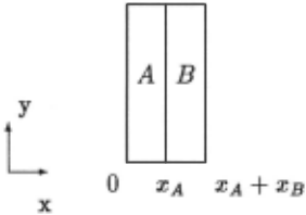
Figure 2: Two Plates Object

A has conductivity of 0.72 Wjm.K, specific-heat of 835 Jjkg.K, and density of 1920 kgjm 3 · Plate B has con­ ductivity of 0.22 Wjm.K, specific-heat of 1085 J jkg.K, and density of 1680 kgjm 3 · Their initial temperature is 273.15 K. They are exposed to an environment of temperature 473.15 K with convection heat coefficient of 50 Wjm 2 .K. The query involves the temperature of both plates with respect to all three spatial dimensions and time, i.e., T(x, y, z, t). The following is a trace of major steps that generates a one-dimensional transient heat transfer model for the composite plates.

1. Preprocessing:

• MSG first identifies a common surface between Plates A and B.
• Thermal Resistances for Plate A, Plate B are 0.091 K.m 2 jW, and 0.028 K.m 2 jW. Ther­ mal resistance for each environment is 0.02 K.m 2 jW.
• Total resistance is 0.159 K.m 2 jW.

2. Choices of Control Regions:

• Since the object is a two-plates object, MSG uses thermal resistance ratios to determine the type of control region in each plate. RA/ Rtotal is equal 0.57 and RB/ Rtotal is equal to 0.18. Both of them are greater than the lumping threshold of 0.1. Differential control regions, evA, evB, are chosen for both plates.

3. Choices of Physical Processes:

• For the differential control region evA, MSG instantiates a set of processes {E,Q:r, ... Qz+dz}, which contains the conduc­ tion processes Q in the x, y, z dimensions and the energy storage process E.
• MSG uses the aspect ratios to estimate the magnitudes of conduction processes in the y, z dimensions. Both the aspect ratios are 0.07, smaller than the spatial threshold of 0.1, MSG removes Qy, Qy+dy, Qz, Qz+dz from the set and reduces the final set of processes to {..E, CJ:r, O:r+d:r}·
• MSG retains E since !:l.T/TreJ = (473.15273.15)/473.15 is larger than the transient threshold.
• Linear properties are chosen for their input val­ ues which are constant.
• Similar choices are made with respect to the control region evB.

4. Mathematical Transformations:

• MSG maps { E, Q :!', Q :r+d:r} into a mathemati­ cal equation Q:r- Q:r+d:r = E for evA.
• Since the query involves temperature, MSG ex­ pands the equation Q:r - O:r+d:r = E into the governing equation shown in Figure 3.
• MSG instantiates an initial condition equation, TA(x, 0) = 273.15 for evA.
• MSG instantiates two boundary condition equations at X= 0, X= xA for eVA.

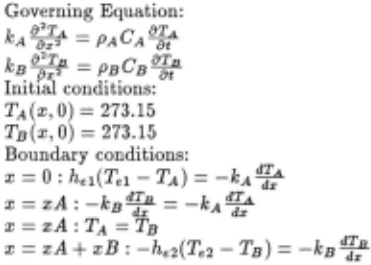
Figure 4: Part of MSG's Actual Output

• Because of a common surface between the plate A and B, MSG instantiates TA = Tn at x = xA.
• Similar steps are repeated for CVn except only one boundary condition is instantiated at x = xA + xB. The boundary condition at x = xA has already been instantiated in the previous step for CVA.

The final model, shown in Figure 3, has two govern­ ing equations (PDE) describing the temperature distri­ bution in the plates in the x direction, four boundary equations for the surfaces of the plates and two initial conditions. Part of the actual output from MSG is shown in Figure 4.

4.2 Implementation and Testing

MSG has been implemented in Common Lisp and CLOS and interfaced with MAPLE, a mathematical manipu­ lation system. The system is able to formulate heat transfer models for single and multiple components of rectangular shape geometries, including composite plates, concentric shell and L-shaped blocks. The sys­ tem has been tested with 27 problems taken from two heat transfer textbooks [Incropera and DeWitt, 1990; Jaluria and Torrance, 1986] and 16 hand-crafted prob­ lems. The textbook problems come from heat transfer analysis in walls, in ovens, in cooling of electronic cir­ cuits and in materials bonding. The list of examples are listed in [Ling, 1994]. The examples cover three kinds of queries. They are: energy storage, heat flux and tem­ perature distribution varying with respect to spatial and time dimensions. The models range from coupled nonlin­ ear three dimensional partial differential equation mod­ els to algebraic equations.

5 Discussion

This section describes several issues and consequences of using a domain theory and problem specific behavior to guide modeling decisions.

5.1 Models Consistent with Domain Theory

Models are not just symbols and equations to produce numerical results. They represent physical realities of a domain. Engineers and scientists use models to obtain numerical data and use the data to guide their activities in physical world, such as planning physical experiments and building artifacts. To be able to use the numeri­ cal data and to have confidence in the data, they must be able to interpret their models as representing valid physical realities according to the theory of a domain. While they are interested in the accuracy of a model, they would also like the model to be consistent with the basic domain theory. Given a choice, they do not want models which just curve-fit the data without relation­ ships to the underlying physics of a domain. The issue is especially important in formulating models in a do­ main with a well-established theory, where models are seen as instances of the theory applied to physical phe­ nomena. However, some approximations, such as the order of magnitude approximation, can lead to approxi­ mate models that are inconsistent with a domain theory, if they are applied to mathematical equations syntacti­ cally. This is illustrated in the following two examples.

In the order of magnitude approximation, a mathe­ matical expression A-B is simplified to A when A~ B, i.e., the numerical value of A is much greater than the numerical value of B where the notion of much greater is defined by some numerical measure.

First Example The first example involves a model rep­ resenting the radiant heat exchange between a sur­ face and its surroundings, shown in the left side of Figure 5. The model is a£(T{ - Ti) where a rep­ resents the Stefan-Boltzmann constant, £ represents emissivity of a surface, T1 the temperature at sur­ face and T2 , the temperature at its environment. Assuming that T{ ~ Ti, then the order of magni­ tude approximation can simplify the original model to a simplified model a£T{, representing a single radiant heat flux emitted from the surface at tem­ perature T1 . The simplified model is consistent with the heat transfer theory.

Second Example The second example involves a model representing the convection heat exchange between a surface and its surroundings, shown in the right side of Figure 5. The model is hA(T1- T2)

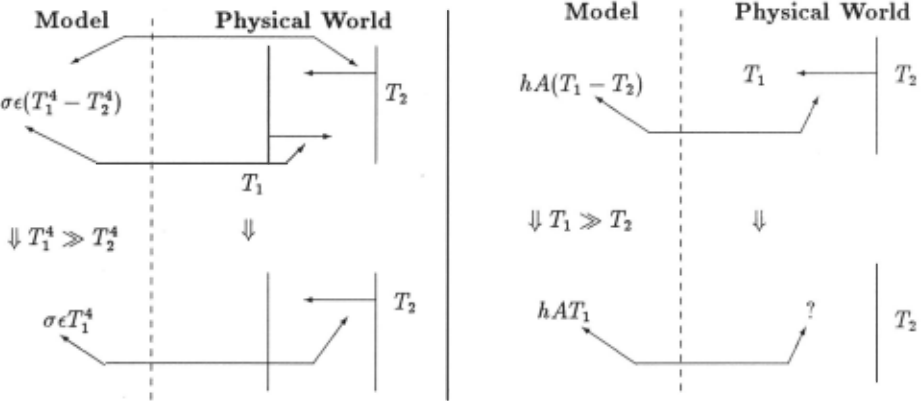
where h represents the convection heat coefficient, A represents the area of a surface, T1 the tempera­ ture at surface and T2 , the temperature at its envi­ ronment. Assuming that T1 ~ T2 , then the order of magnitude approximation can simplify the model to a simplified model hAT1 · However, that simplified model is not consistent with the heat transfer the­ ory as the expression does not represent any valid heat transfer process. The original model represents a convection heat flux and eliminating T2 from the original model destroys its definition, i.e., convec­ tion heat transfer depends on temperature differ­ ence instead of temperature only.

The two heat transfer examples illustrate the case where the syntactic use of the order of approximation can lead to approximate models inconsistent with a do­ main theory. To ensure models consistent with a domain theory, the order of magnitude approximation cannot be applied to any arbitrary mathematical expression. It can only be applied to a set of physical processes in a way that represents the action of eliminating one or more physical processes. By focusing the approximations on choosing the types and the number of physical processes in a domain, MSG avoids generating models inconsistent with the heat transfer theory. The constraint of ensuring consistent models is already built in MSG.

5.2 Constraining Modeling Process

MSG demonstrates that the process of modeling is com­ positional at the level of choosing physical processes. Furthermore, it demonstrates that a domain theory can constrain how modeling decisions are made. Some mod­ eling decisions can only be made after other decisions have been made. For example, formulating boundary conditions has to be made after choosing physical pro­ cesses, and choosing physical processes has to be made after choosing control regions. A consequence of con­ straining modeling decisions is that modeling choices are also constrained by the earlier decisions, leading to a reduced search space for MSG. If a totally lumped control region is chosen, MSG does not need to choose heat transfer processes since a totally lumped model will only involve an algebraic or ordinary differential equa­ tion, either of which can be efficiently solved with many processes. Furthermore, MSG does not need to choose boundary equations for the totally lumped model. The reduced search space from constraining modeling deci­ sions, and the use of simple approximate model to guide modeling decisions contribute to the efficiency of MSG. MSG currently takes less than 4 seconds on a SparcSta­ tion 2 to formulate a model involving coupled partial differential equations.

MSG demonstrates an uniform approach to formu­ lating models of various complexity in a physical do­ main, from simple algebraic to complex partial differen­ tial equations models. While partial differential equa­ tions are complex to analyze and difficult to compre­ hend, they are formulated in the same way as other sim­ ple models. They do not need a different modeling ap­ proach. The complexity of a model lies not in the way it is formulated, but in the choices made to the physical processes.

5.3 Limitations

This approach works because of a strong domain the­ ory, where conservation laws exist and the domain spe­ cific laws are well defined, and approximate numerical methods and thresholds calibrated against accuracy are available. These features are present in other domains as well, such as fluid mechanics [Panton, 1984], based on textbook analysis and discussions with domain experts. However, the requirement of a strong domain theory and the availability of approximate methods and thresholds limit this approach to well-established physical domains.

6 Related Work

Yip [Yip, 1993] uses the asymptotic order of magnitude approximation to simplify partial differential equation models in fluid mechanics. His system accepts a de­ tailed mathematical model and the constraints and val­ ues of terms in the model as inputs, and then carries out the asymptotic order of magnitude approximation on the input model. MSG differs from his system by using ap­ proximate models to infer the order of magnitude values of physical processes and by carrying out approximations on physical processes to ensure models consistent with a domain theory.

Most of the other modeling work is based on the com­ positional approach pioneered by Falkenhainer and For­ bus [Falkenhainer and Forbus, 1991]. The compositional approach has a library of model fragments represent­ ing various phenomena in a domain. Given a query and a physical situation, the approach composes relevant model fragments into a complete model. Other work [Iwasaki and Levy, 1994; Nayak et al., 1992] has proposed ways to improve the process of selecting model frag­ ments. MSG differs from the compositional approach by focusing its modeling decisions on physical processes and using a domain theory to structure its modeling pro­ cess. By organizing its modeling decisions around a do­ main theory, MSG can formulate models for lumped and distributed phenomena in an uniform and efficient way. The compositional approach is aimed at a very broad class of phenomena, without making any assumption of a domain theory. MSG relies on a strong domain the­ ory, which makes MSG less broadly applicable than the compositional approach, especially for a domain with no well developed theory. The compositional approach can handle qualitative and quantitative ordinary differential equations. MSG is focused on quantitative models in­ volving algebraic, ordinary and partial differential equa­ tions. Finally, the compositional approach has paid less attention to the issue of getting the right level of nu­ merical approximation than to getting a consistent and coherent model.

Both Addanki et al [Addanki et al., 1991], Ellman et al [Ellman et al., 1993] and Weld [Weld, 1992] focus on model selection. The work of Addanki et al uses graphs to represent a set of models of a physical domain, and do­ main specific rules to select models that can resolve the conflicts between predictions and observation. Weld's work uses the domain independent technique of inter­ model comparative analysis. Ellman et al use gradient magnitudes to select models. In all cases, model equa­ tions are explicitly input to the system. MSG differs from them by constructing a model from the description of a physical phenomenon.

7 Summary

This paper describes a modeling approach to formulating complex mathematical models involving partial differen­ tial equations. The approach is targeted to domains with strong domain theories. The approach organizes its mod­ eling process based on the structure of a domain theory, and uses simple approximate models to obtain problem specific behavior to guide its modeling decisions. By ex­ ploiting these ideas, the approach can offer an uniform and efficient way to formulate models consistent with a domain theory. The approach has been implemented in a computer program, MSG, which formulates algebraic, ordinary and partial differential equation models in the domain of heat transfer.