Case-based Modeling with Qualitative Indices

1 Introduction

Understanding physical systems well enough to predict and control their behavior has long been a goal in engin­ eering and science. When systems are simple, numerical equations can exactly reproduce the system's behavior. For complex systems, however, developing an accurate numerical model is rarely feasible.

Qualitative modeling alleviates this problem by model­ ing systems at a higher level of abstraction. A qualitative model seeks to identify and model only the most import­ ant aspects of a system. In the classic example of a ball thrown into the air, an abstract model will not attempt to predict how high the ball rises-but only that it will rise to some height, reverse direction, and fall to the floor.

Qualitative modeling techniques such as QSIM [8] and qualitative process theory [3] have been success­ ful at modeling complex physical systems at this level. However, predictions at the qualitative level are insuffi- Peter Duxbury-Smith NESTEC YORKRECO P. 0. Box 204 York Y01 1XY, Great Britain 100105.1166@compuserve.com ciently precise for tasks that do require numerical res­ ults, such as diagnosis and process control. Techniques such as Q3 [2] SQDE [7] and SIMGEN allow combining the qualitative models with numerical equations to obtain precise results. However, such techniques are applicable only when these numerical equations are known, again restricting them to well-understood processes.

For many practical systems, this is not the case. For example, the tests in this paper were carried out on a coffee roaster, used in various plants of Nestle, for which it has so far been impossible to construct an accurate nu­ merical model. The absence of accurate numerical pre­ dictions has led to many critical situations , such as fires , which destroy the entire load of coffee beans and require expensive shutdowns. Since prevention of these critical situations depends on the numerical prediction of key parameters, purely qualitative models are insufficient .

However, an enormous amount of information about the roaster is available in the form of records of past be­ havior. An alternative to generating a numerical model is to use case-based reasoning, where predictions are based on previous experiences. Marc Goodman [5) has repor­ ted promising results using this paradigm to make pre­ dictions about the behavior of a complex video game.

The major problem for such an approach is indexing: which of the wealth of previous observations are in fact relevant to the current situation? In this paper, we de­ scribe two ways in which a qualitative model can be used to provide such indices, allowing us to combine past ex­ periences into a prediction for the current situation.

A first approach to locating relevant precedents is nearest-neighbor search. Here, the problem is to find an appropriate similarity metric which assigns weight to those aspects which are important for the prediction. We have implemented a system where this metric is determ­ ined based on a qualitative model, and tests on actual coffee roaster data have shown satisfactory results.

In another approach, first mentioned by Hellerstein [6), the qualitative model is used to determine which exper­ iences can provide bounds on the current situation. We have also implemented this second approach and have obtained very promising results.

When prediction concerns a commonly occurring situ­ ation, it is usually possible to locate a single almost identical past experience that gives the correct predic­ tion. However process prediction is most important in critical situations for which past experience is (hopefully) sparse. A prediction may then have to be construed from several precedents, none of which is entirely similar to the current situation. More precisely, each parameter may be predicted from cases selected according to cri­ teria specific to that parameter. Our approach is capable of intelligently combining information from several cases into a single solution.

Using records of historical behavior to provide quant­ itative information has the marked benefit that the in­ formation is "free". In other words, where development of a numeric model requires a great deal of effort, de­ veloping a library of cases requires only that we monitor the system and record what it does-something that is a normal part of most process-control systems.

Our techniques offer two further benefits. First, when dealing with complex machines, each machine may well have its own individual characteristics within some range of "normal" behavior. By using cases recorded from each machine, we automatically account for these indi­ vidual variations. Second, although our techniques take as input qualitative information about the system, they do not require this information to be complete or correct; accuracy degrades gracefully as the qualitative model de­ teriorates.

2 Background

Qualitative models are descriptions of a system stated in non-numeric terms. The formalism we use is that of QSIM 1 , in which a model consists of a set of qualitat­ ive constraints. A qualitative constraint represents an unknown numeric function which holds amongst the ref­ erenced variables. For example, the constraint M+(a, b) states that a strictly monotonically increasing function holds between variables a and b, although the exact func­ tion is unknown.

The problem we seek to address is that of process pre­ diction and control. Performing process prediction is a precursor to addressing the process control problem. The problem of process prediction may be stated as:

• Given: the current state of a system, given by the numerical values of a set of parameters (and possibly recent historical information).
• Predict: the state the system will be in at a spe­ cified time in the future, again expressed as the nu­ merical values of a set of parameters.

In this paper, we limit our attention to the problem of process prediction. Process control requires taking corrective action once prediction shows that an undesir­ able state is about to be reached. Determining appro­ priate control actions will require additional knowledge about the effects of control parameters on system vari­ ables. The idea of augmenting a qualitative model with case-based reasoning may be more difficult to apply to control actions, since historical data about corrective ac­ tions is scarce.

1 But most other formulations are equivalent for the pur­ pose of this application.

Without loss of generality, we consider predicting only a single parameter at a time; we call it the query para­ meter. Predicting the entire state can be carried out by repeatedly applying the procedure to each parameter in the state description.

The application we are using is a continuous-roast cof­ fee roaster used by Nestle. The problem underlying cof­ fee roasting is that it is exothermic, and thus inherently unstable. The continuous-roast devices are a new tech­ nology, and the theoretical specifications of the machines (stated as numerical equations, etc.) have proven inad­ equate as a basis for process control. The result is that the machines must often be shut down, because the pro­ cess is leaving its normal operating region and cannot be brought back by the current control system.

In this application, the process monitoring logs con­ tain snapshots taken of the system every thirty seconds. Each snapshot records the values of 60 parameters. His­ torical cases are provided in the form of one or more such process logs, each containing approximately 24 hours of data (about 2800 snapshots). In the results presented in this paper, we are trying to predict system behavior 10 minutes, or 20 samples, ahead.

The qualitative model represents the known relations between these roaster parameters. An important advant­ age of the qualitative model is that it does not have to be complete, and some relations may be missing without rendering it incorrect . Our hand-built model contains known simplifications and approximations of the pro­ cesses taking place within the roaster.

3 Adaptation of historical cases

The techniques we use for prediction were originally de­ signed to predict missing feature values from static cases (the traditional task performed by many case-based­ reasoning and machine-learning programs). In order to perform prediction, we first must adapt the cases to the prediction task.

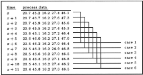
Our approach is to take the process monitoring logs and create cases which combine information from differ­ ent times in the process log. So, for example, if we are predicting 6 samples into the future, each case consists of two time points from the process log: one from timex and one from time "x + 6" (see Figure 1).

The system's current state provides us with the left­ half of a case, and we use our constructed library to estimate the values that should appear in the right-half. The prediction problem is thus reduced to the betterunderstood problem of predicting missing values (albeit continuous values, which is not possible using many ma­ chine learning techniques).

4 Direct prediction

Our first approach, described originally in [11], performs direct prediction. We take as input a QSIM model of the system, and use this to determine, for each parameter, which other parameters should be used as a basis for prediction.

In [11] we wanted to solve a qualitative model as set of equations; the end result was to be stated in terms of a few distinguished variables. In the prediction task, however, all variables which appear in the logs are equally available, so none are distinguished. This makes the equation-solving trivial, and results in useless case indices (the indices devolve to the variable appearing in the first constraint to reference the target parameter) .

However, equation solving can be viewed as graph tra­ versal, where we are tracing paths to some set of distin­ guished nodes. In the prediction problem, where most or all nodes are distinguished, we need an alternate heur­ istic. The heuristic we use here is the following: the case indices for a parameter is the set of all variables in the model-graph which are distance d from the parameter, and dis a user-selectable integer greater than zero.

The intuition behind this selection is that causality must flow through the system in some direction. While the qualitative model does not provide any information on causality, one or more of the parameters nearby in the model-graph should be predictive. And we have elimin­ ated many "distractor" parameters, which would be ir­ relevant or possibly damaging to the prediction accuracy. The algorithm for model-based prediction is:

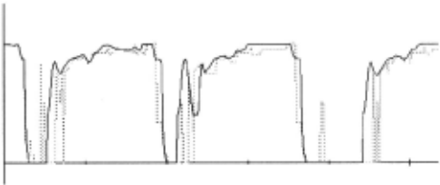
For each parameter we are to predict Determine indices For each timepoint Select the nearest case or cases Take the predicted value from the selected cases end for end for

Given the indices, we use a simple nearest neighbor (lNN) matching method; while more sophisticated meth­ ods are available, using a simple method provides with the best feedback on the efficacy of our indexing tech­ nique. A sample prediction graph appears in Figure 2. Here, the dotted line represents the predicted values, whereas the black line shows the actual system behavior. Tics on the X-axis represent fifty-minute intervals.

5 Bounding behaviors

The second approach we present is based on [6]. This approach determines experiences that provide upper and lower bounds on the value of a query parameter P based on the following consideration. Assume that P is related to other parameters Q and R by the constraints M+(P,Q) and M-(P,R). These constraints can be used to partition the set of previous experiences into three sets:

• (Qprecedent :::; Qactuaz) I\ (Rprecedent ~ Ractuat) : Pprecedent :::; Pactual is a lower bound for P.
• (Qprecedent ~ Qactuat) I\ (Rprecedent :::; Ractuat): Pprecedent ~ Pactual is an upper bound for P.
• others: irrelevant for bounding Pactual ·

If the qualitative model were perfectly accurate, system behavior completely consistent, and measurement noise negligible, then the greatest lower and smallest upper bound would provide a precise interval within which the actual value of P must fall. In practice, various inac­ curacies mean that the measured behavior is typically normally distributed over an interval. Hence, we ask the use to provide a desired confidence level, and then use statistical techniques to determine upper and lower bounds for the confidence interval, as described in (6] ..

The set of related variables and their qualitative rela­ tions is obtained by taking the transitive closure of all M+ and M- constraints present in the qualitative model. Since the parameter being predicted also appears in the historical portion of the case, we automatically add a positive monotonicity relating the parameter to itself. If the qualitative model is reasonably complete, there will typically be several related variables, thus providing a strong index where only a small fraction of the previ­ ous experiences will be relevant to an actual prediction problem. The algorithm for this approach is:

Sort all cases by nearness to the current case For each parameter we are to predict Determine the upper bound:

Find theM nearest cases which are ''above'' the current case Sort the M values taken from these cases Select the upper bound, based on the desired confidence level Determine the lower bound: Find theM nearest cases which are ''below'' the current case Sort the M values taken from these cases Select the lower bound, based on the desired confidence level

end for

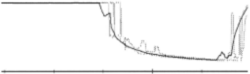
One limitation is that the confidence level depends on cases being randomly selected from a normally distrib­ uted population. Since our cases are taken from temporal sequences, they are not independent (although we do use multiple, independent sequences). This means that the true statistical confidence may not correspond to that selected by the user; however, this has not proven to be a problem in practice. Figure 3 shows a sample predic­ tion made using this approach. The dotted lines show the bounds of the confidence intervals, and the black line shows the actual values.

6 Empirical results

This section presents our empirical results in four sec­ tions, followed by a fifth section discussing the results of the model-based algorithms. The empirical tests were:

• tests showing how accuracy is affected by removing "redundant" data from the case base
• standard learning curves, showing the prediction ac­ curacy of various methods
• model dependence tests, showing how accuracy IS affected as the qualitative model degrades
• prediction period tests, showing how accuracy changes as we predict farther ahead in time

We selected five data files to use in all tests; logs from one roaster taken from five days in January 1994. In all cases, the roaster was producing the same recipe, which means that the external settings were identical. All logs contain one or more anomalous events; normally emer­ gency shut-downs followed by some period of inactiv­ ity and a process restart. Depending on the test, we use between one and four logs as the source of histor­ ical cases, and one as a test set. Each data point in the graphs that follow represents the average of five test runs, one using each of the logs as a test set.

The confidence for the bounding approach was set to 90%, meaning that on average 90% of the predicted val­ ues fall within the predicted bounds. As a basis for comparison, we also include results using the IB1 al­ gorithm [1], which indexes on all parameters. Except for line-crossings, all results are statistically significant (p ::=; 0.01). However, since we are drawing data from temporal sequences, case selection is not truly random; this means that the value calculated for statistical signi­ ficance should be taken only as a general indication.

6.1 "Forgetting" redundant data

In practice, a systemlearns as more experiences are ad­ ded to its database. However, since memory and indexing capabilities are limited, we must provide a method for re­ moving redundant data. In practice, much of the roaster data simply represents normal operation, with all values varying over relatively small ranges. Having hundreds of hours of such data on-line is not really very useful. Hence, we have implemented a filtering algorithm that deletes redundant cases.

To identify redundant cases, we first determine the range over which each parameter varies. We say that some second case is redundant (and can be eliminated) if every parameter is within r% of the range of the corres­ ponding parameter in the first case. For example, sup­ pose we have cases containing only the single parameter x, which varies from -5 to +5. If the user specifies a redundancy level of 15%, then two cases would be con­ sidered redundant if: abs(x1 - x2 ) ::=; 1.5.

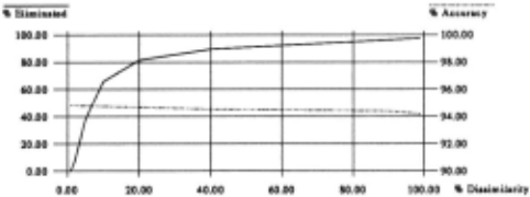
To our surprise, even relatively harsh filtering, with r over 90%, did not have a severe impact on predict­ ive accuracy. When using four days of data, we began with about 10,000 constructed cases; after filtering at 90%, we were left with about 300 cases, which were then evidently sufficient to cover the range of roaster beha­ vior with reasonable accuracy. We do not yet know if this relative insensitivity is application specific; our fu­ ture work will certainly include testing this on other real data sources. Figure 4 shows the reduction in case size realized by various values of r, along with the accuracy impact when using the IB1 algorithm; the accuracy of model-based prediction behaves almost identically.

6.2 Learning curves

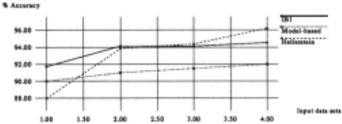
Figure 5 shows a standard learning curve for prediction using the IBl algorithm and using the model-based al­ gorithms. These learning curves were produced using a similarity reduction r of 40%, except that no reduction was done on data provided to the bounding approach. The reason for this is that the statistical derivation pro­ cess depends on the presence of redundant information in the database.

As can be seen, the model-based prediction algorithm did not perform as well as simple IBl. Given the good results seen in [11], we were surprised at this result, and it led to the analysis discussed in Section 6.5. However, it is worth noting that the accuracy is competitive, and that the smaller indices used in the model-based approach yield much faster execution times.

To allow direct comparison of all approaches, we have also graphed the Hellerstein approach in Figure 5. However, interpretation of this requires some caution, as this algorithm is not attempting to do direct prediction. The "accuracy" in this case is the average distance of the upper and lower bounds from the actual value (hence, if the upper and lower bounds were simply the highest and lowest possible values, the "accuracy" would be 50

This means that the "accuracy" of the bounding ap­ proach actually represents the tightness of the confidence interval. Thus, the graphs show that the bounds are as tight as the error of the directly predictive approaches­ this in spite of· the fact that these are outer bounds on possible behavior. However, the projected bounds are, in some sense, more useful. Whereas a projected value is either right or wrong, the bounds tell us a range in which the value will fall, with some degree of certainty­ and we can raise the degree of certainty as high as we like simply by collecting more data.

The chief disadvantage of the bounding approach is that, to achieve high statistical certainties, we must re­ tain redundant data in the database- reducing the effi­ ciency of the approach considerably. One could envi­ sion an approach whereby one tagged retained cases ac­ cording to how many similar cases had been "forgotten". This "weighting" of individual entries in the data base would allow one to approximately reconstruct the ori­ ginal statistical population without having to remember all cases.

6.3 Model dependence

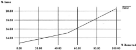
To verify our hypothesis that our approach degrades gracefully with the quality of the input model, we ran a test in which we gradually removed constraints from the model (see Figure 6). This test was done using the bounding approach. Since the presence of large amounts of data tends to improve performance the performance of poor indexing schemes (given enough examples, even a poor indexing scheme will find an applicable example), we emphasized the model's importance by only using a single historical data set in each test run.

As constraints were removed from the model, the width of the bounds (graphed as "error") does indeed increase, but it does so gradually. Ultimately, when all constraints are removed, the only remaining index is the variable itself; prediction of the query parameter's future value is based solely on its past value, resulting in a confidence interval with an average width of more than 40% of the parameter's range (each bound is, on average, more than 20% distant from the center point) .

6.4 Prediction period

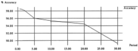
Finally, we were curious to see how far into the future we could predict system behavior . Using the IBl approach with the reduction parameter set to 90%, we measured predictive accuracy out to 30 minutes (60 samples) (see Figure 7) . As expected, predictive accuracy is highest when predicting only a very short distance into the future. However, accuracy remains quite good through 20 minutes ( 40 samples) .

6.5 Analysis of model-based results

The disappointing results of direct model-based predic­ tion led us to analyze the predictions being made. One of the major problems appears to be the lack of times­ cales in the model. For example, if the burner setting in the roaster increases, we can expect an increase in the furnace temperature after a few seconds-and this rela­ tionship is reflected in the model. However, there is no such direct relationship when predicting 10 minutes in the future.

To improve the model-based results, we need to de­ velop a qualitative model for the timescale at which we are doing predictions. However, since the system we are working with is, in fact, very poorly understood, it is not clear what such a model should look like. Hence, we are now working on methods to derive a partial model dir­ ectly from this historical data, using techniques drawn from [12] and other sources.

The bounding approach is evidently less sensitive to these problems in the model, probably because it collects a statistical sample of cases from which it derives its bounds. However, we would expect its performance to improve as well , given a model suitable for the timescale at which we are doing prediction.

7 Related work

In this paper, we presented two approaches for combining qualitative models with historical behaviors, for the pur­ pose of doing prediction. The first of these approaches, model-based indexing, is based on [11]; however, in [11], this technique was used to develop process settings in terms of desired process outputs and ambient conditions, a well-defined subset of the process variables. In predic­ tion there are no such distinguished parameters, so the approach was altered to use all parameters within a cer­ tain distance of the query parameter. In our test domain, this turned out not to work as well as we hoped. Since the results in [11] are quite good, we believe this is due to the model-timescale problems discussed above.

Our second approach was based on [6], which uses his­ torical information to develop confidence intervals for the values of unknown parameters. We were able to adapt this approach directly to the task of process prediction, and the tightness of the confidence intervals is compet­ itive with the accuracy of purely predictive approaches, which we consider an very positive result.

An alternate approach to combining model-based and instance-based learning can be found in [9]. Quinlan uses a quantitative model to correct the values retrieved by a normal case-based system, by applying the model both to the target instance and to the retrieved instance. His idea is that one can use the model to calculate a corrective factor, which is applied to the retrieved in­ stance. This approach works well with a good quantit­ ative model, but, in domains with weak models, the cor­ rective factors proved counterproductive. Our approach, on the other hand, requires only a qualitative model, and uses -the model , not to correct the cases, but to develop indices indicating which cases are most relevant to the current situations.

A number of people in the qualitative modeling com­ munity have added quantitative information to qualitat­ ive models. In [4], Forbus and Falkenhainer use qual­ itative envisionment combined with numerical modeling information; this approach can work well, but requires that one provide both the qualitative and numerical mod­ els up-front . Kay and Kuipers, in [7] take the approach of quantitatively constraining function envelopes, but again this requires numerical modeling information as input.

A different approach to prediction is presented in [5]. Goodman's approach is a combination of inductive learn­ ing and case-based reasoning. He analyzes process logs offline to build clusters of similar behaviors, which are used as the basis for prediction. His approach makes pro­ vision for the addition of qualitative information (prin­ cipally in the form of causal links), but no information is yet available on the accuracy of his predictions or on the effect of adding the qualitative information.

Finally, where do we obtain the qualitative model used to guide the prediction process? In our application, the model was hand-built , and is known to be incomplete. In general , human experts can provide more complete models , but perfect models are generally not available. For this reason, plus the need for timescale-specific mod­ els, we are now looking at the possibility of deriving the needed model directly from the historical records of sys­ tem behavior . The basic techniques needed have already been developed in MISQ [12], [10].

Since some system knowledge is usually available, the model-building process could start from an initial hand­ generated model, and refine it as needed to match the historical observations. This would result in a more dir­ ected and efficient model-generation process. In fact, subsequent errors in prediction could be fed back into the model-generation process , leading to an interesting synergy between machine learning and case-based reas­ oning in this framework.

8 Conclusions

For many physical devices of great economic importance, no accurate mathematical models exist. In some cases, it is in fact questionable whether numerical models of reas­ onable size could ever be constructed, since their com­ plexity means that the number of state variables could be enormous. Occasionally, techniques such as neural net­ works can be used to learn satisfactory prediction mod­ els, but cannot guarantee correct results in all cases.

For most systems, the designers can provide at least a partial qualitative model, which one could enhance using automated model-building techniques. Combining this qualitative model with records of historical behavior, we are able to provide accurate numerical predictions. The fact that predictions are based on a qualitative model provides an advantage over pure statistical techniques (such as neural networks), in that the results can be guar­ anteed to be accurate within reasonable bounds.

Furthermore, even when the qualitative model is in­ complete, our experiments have shown that predictive accuracy degrades gracefully. This robustness stands in contrast to techniques based only on models, where an incomplete model results in an explosion of ambiguities, and model errors can lead to completely wrong conclu­ swns.

We believe that our approch points out an interesting direction for resolving the knowledge engineering bot­ tleneck. Purely syntactic case-based reasoning is often insufficient to cover all situations in complex systems. Model-based reasoning requires a complete and accurate model which is costly to build. By combining the two techniques, we no longer require a 100 % accurate and complete model, but can nevertheless adapt and combine previous cases to achieve good coverage of behaviors with relatively few cases. This disproves the popular myth that case combination and adaptation necessarily rein­ troduces the knowledge engineering bottleneck; on the contrary, model- and case-based reasoning complement each other very well .

Many open issues for further work have become ap­ parent . The first concerns the development of the qual­ itative models. Preliminary work in this area, such as MISQ, has shown that it is possible to develop and refine models from records of process behavior. As the systems collects more and more experience, it should gradually improve its qualitative model through inductive learn­ ing techniques, thus improving its indexing accuracy and ability to handle large and larger databases . However, these automatic model-building techniques need further work before they can be used with real-world systems.

Our results on "forgetting" redundant information also indicate a need for further work. By using a relatively simple heuristic for identifying redundant cases, we were able to eliminate more than 95% ofthe historical informa­ tion without severely affecting predictive accuracy. If this proves not to be application specific, then more sophisticated heuristics should yield even better results. Given the massive amounts of information which are collected through process monitoring, "forgetting" techniques are essential to identify the useful information that should be retained for future reference.

The techniques we have described in this paper have been implemented in C++ under DOS/Windows. We are currently investigating new applications where pre­ diction is important, such as load prediction in power distribution networks.