
Trading off the Costs of Inference vs. Probing in Diagnosis
Proceedings of the Fourteenth International Joint Conference on Artificial Intelligence. Qualitative Reasoning and Diagnosis. Pages 1736-1740.
© 1995 International Joint Conferences on Artificial Intelligence
Abstract
This paper proposes a new algorithm which when provided the relative costs of computation vs. probing minimizes the total cost of diagnosis. During the diagnosis process the decision of whether to probe or to compute is dependent on the expected costs and benefits of each alternative. It is unlikely that we will be able to find general analytic and simpleto-compute models for the costs and benefits. Therefore, we base our algorithm on simple empirically derived models of costs and benefits. With these models, our algorithm operates by continuously choosing the optimum action to make next. This algorithm will not blow up on the rare pathological cases and will always (on average) find diagnoses at equal to or better cost than a conventional GDE/Sherlock. When the cost of probing is high, then our algorithm behaves exactly the same as GDE/Sherlock. When the cost of computation is high, the algorithm performs the diagnosis at far lower cost than GDE/Sherlock.
- Bakker, R.R., and Bolurseau, M., Pragmatic rea- soning in model-based diagnosis, in: Proceedings ECAI-92, Vienna (1992).
- Brglez, F. and Fujiwara, H., A neutral netlist of 10 combinational benchmark circuits and a tar- get translator in FORTRAN, distributed on a tape to participants of the Special Session on ATPG and Fault Simulation, Int. Symposium on Circuits and Systems, June 1985; partially characterized in F. Brglez, P. Pownall, and R. Hum, Accelerated ATPG and fault grading via testability analysis, Proc. IEEE Int. Symposium on Circuits and Sys- tems, (June, 1985) 695-698.
- Boddy, M. and Dean, T., Solving time-dependent planning problems, in: Proceedings IJCAI-89, De- troit, MI (1989) 979-984. IJCAI
- de Kleer, J. and Williams, B.C., Diagnosing mul- tiple faults, Artificial Intelligence 32 (1987) 97- 130. Also in Readings in NonMonotonic Reason- ing, edited by Matthew L. Ginsberg, (Morgan Kauf- mann, 1987), 372-388. Also in [12).
- de Kleer, J. and Williams, B.C., Diagnosis with be- havioral modes, in: Proceedings IJCAI-89, Detroit, MI (1989) 104-109. Also in [12). IJCAI
- de Kleer, J ., Raiman, 0. and Shirley, M.H., One step lookahead is pretty good, in: [12)138-142.
- de Kleer, J ., Focusing on probable diagnoses, m: Proceedings AAAI-91, Anaheim, CA (1991) 842- 848. Also in [].
- de Kleer, J. and Raiman, 0., How to diagnose well with very little information, in: Proceedings of the Fourth International Workshop On Principles of Diagnosis, Aberystwyth, Wales (1993) 160-165.
- de Kleer, J., A hybrid truth maintenance system, forthcoming.
- Forbus, K., and de Kleer, J ., Building Problem Solvers, MIT Press, Cambridge, MA (1994).
- Friedrich, G., and Nejdl, W., Choosing observa- tions and actions in model-based diagnosis-repair systems, in: Proceedings KR-92, Cambridge, MA (1992) 489-498.
- Hamscher, W., de Kleer, J., and Console, L. (eds), Readings in Model-Based Diagnosis, Morgan- Kaufmann, 1992.
- Horvitz, E.J ., Breese, J ., and Henrion, M., Deci- sion Theory in Expert Systems and Artificial Intel- ligence, Technical Report KSL-88-13, Stanford Uni- versity Knowledge Systems Laboratory, February, 1988.
- Horvitz, E.J ., Reasoning under varying and uncer- tain resources constraints, in: Proceedings AAAI- 88, Saint Paul, Minn. (1988) 111-116.
- Nejdl, W., and Bachmayer J ., Diagnosis and repair iteration planning versus n-step lookahead plan- r.ing, in: Proceedings of the Fourth International Workshop On Principles of Diagnosis, Aberyst- wyth, Wales (1993) 121-135.
- Russell, S. and Wefald, E., On optimal game-tree search using rational meta-reasoning, in: Proceed- ings IJCAI-89, Detroit, MI (1989) 334-340. IJCAI
- Sun, Y., and Weld, D., A framework for model- based repair, in: Proceedin!Js AAA.f-.9J', Washing- ton, D.C. (1993) 18'2-187.
References were extracted automatically from the PDF and may contain errors.
Full text extracted automatically from the PDF; figures, tables and equations may differ. The PDF is the version of record.
1 Introduction
A key goal of the diagnostic task is the identification of which component malfunctions are causing the unde si rable symptoms. Recently there has been a consider able amount of exploration of the task of restoring the device to correct functioning at minimal cost [11 ; 15; 17]. Much of this research is aimed at minimizing the total cost of probing, repairing, and downtime. For ex ample, the decision of whether to repair or to probe is dependent on the relative costs of probing vs. repair ing. There has also been a considerable amount of effort into designing better diagnostic algorithms [7]. Although these algorithms have made model-based diagnosis far more practical, their design goals have been to produce faster algorithms without concern about the tradeoff of inference time vs. other costs. In this paper we ex plore the tradeoff between inference and probing costs and propose a new algorithm which when provided the relative costs of computation vs. probing minimizes the total cost of diagnosis.
There are three basic reasons why it is important to take into account computation time. First, no mat ter how good the algorithm, there are devices and in puts that require an inordinate amount of computation. When faced with these rare, but nevertheless very real , cases many algorithms fail to provide useful diagnoses within reasonable time . . Second, the relative costs of computation and probing vary tremendously in applica tions. In one application, almost every signal can be measured immediately. In another application, measur ing a signal may require sending a technician a mile down a mine shaft. On the other hand, some applications have enormous computational resources available, while in others the amount of computational resources avail able is minimal. Finally, even if computation could be regarded as "free," downtime to the customer often is not . The cost of the computation is often not the actual CPU charges, but the cost during which the customer's system is nonoperational.
2 The GDE/Sherlock Framework
We adopt the model-based diagnosis framework of GDE/Sherlock [4; 5]. A typical GDE [10] implemen tation consists of a constraint propagator (constraints are typically used to model the components) and an assumption-based truth maintenance system (the ATMS is used to record assumptions) . GDE operates as follows:
- Using the constraint propagator and the ATMS, identify all (preferably minimal) conflicts (a con flict is a set of components, at least one of which is faulted). The conflicts are represented as ATMS nogoods.
- From the conflicts, construct all diagnoses.
- Given all the diagnoses, determine the optimal probe.
The sequence of computation and probing can be illus trated by Fig. 1. Only by determining all the diagnoses first can GDE produce the optimal sequence of probes.
Sherlock [7] is a far more efficient diagnostic algorithm, upon which we base our new algorithm. The first two steps of the GDE algorithm are inherently exponential. We can remove much of those exponentials by observ ing that most diagnoses (the low probability ones) have an insignificant effect on probe selection and most con flicts are irrelevant for determining those diagnoses. By focusing the ATMS (an HTMS [9]) we avoid ATMS la bel explosion. Sherlock operates roughly as follows (for more details see [7]):
- Perform a best-first search (using prior probabili ties) to find a candidate diagnosis which does not subsume any of the currently known conflicts.
- Use the constraint propagator and the HTMS to test whether the candidate diagnosis is consistent with the observations. If it is not, then find one conflict which subsumes it and add it to the current known conflict set, and return to step 1.
- Save the new diagnosis, compute its relative poste rior probability via Bayes Rule .
- If the cutoff criteria is not me, then go to step 1.
- If we have one diagnosis, we are done.
- Perform the best probe, based on the diagnoses so far. Go to step 4.
In the situation (which we explore in this paper) where most diagnoses have similar probability, the probe compute profile of Sherlock is no different than that of GDE (Fig. 1). We propose that computation and prob ing be intermixed (illustrated in Fig. 2). Intermixing computation and probing will clearly increase the to tal amount of probing-probes will be selected with less available information about the space of possible diag noses. What may not be as obvious is that this inter mixing will decrease overall computation time. When the probabilities of diagnoses vary significantly, Sherlock will also intermix computation and probing because if all current diagnoses are eliminated, it will return to step 1. But this is ad hoc - our new algorithm will make the decision of whether to compute or probe on a principled basis.
In Sherlock, every candidate diagnosis has to be checked and eliminated (in step 1 or step 2) . The fact that computation and probing are intermixed does not reduce the total number of candidates that have to be checked. Computation time is improved because candi dates can be eliminated far more quickly if more infor mation is known about the faulty device. A probe may yield a new conflict which can easily eliminate a large number of the candidates in step 1. If a particular can didate is not subsumed by a conflict, it still needs to be checked to see whether it gives rise to new conflicts in step 2. Every new probe made of the device, in essence, splits the device into two or more pieces. Thus the test of a new candidate is much less expensive. So the ba sic advantage of intermixing computation and probing is that the same computation task will become cheaper once more is known about the device.
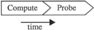

Steps 1 through 3 above form an anytime algorithm it can be stopped at any time and provide a current list of valid diagnoses in decreasing probability order and the accuracy of this diagnosis set increases monotonically. Steps 2 and 6 consume all the cost, so we will modify the algorithm to do a cost-benefit analysis at those points to decide whether to probe or to compute. The resulting algorithm will be described later.
In order to simplify the analysis we make a number of assumptions about the nature of the diagnosis task:
- Costs of all probes are constant and equal. This can be relaxed somewhat by introducing multi-step lookahead; but we do not explore this issue in this paper. If probe costs vary, then the decisions made by the algorithm may not be reasonable.
- The cardinality of the diagnoses is presumed to be constant. In other words, we do not expect the car-
dinality of the diagnoses being considered to change during the diagnosis session. (For example, we can not handle the case where all singlefaults are elim inated, and then doublefaults are considered. Our proposed algorithm will suggest suboptimal probes in this case.)
3 Benefit of Knowing Another Candidate
GDE/Sherlock's algorithm searches the diagnostic space in a fixed order. It yields the diagnoses in decreasing probability. At any point the search can be suspended and restarted. The basic question we need to answer is the relative value of finding a next candidate. That value will be the number of fewer measurements the al gorithm will have to make given that we know that can didate. This is not easy to estimate. GDE/Sherlock can not easily provide the number of diagnoses that explain the symptoms before the cutoff criteria will be met 1 , nor what their probabilities. Hence, we have no information about the number of diagnoses that might exist. To truly make the optimum next probe requires knowing all the diagnoses. Perhaps there is some analytic formulation of the number of candidates, but we have not been able to construct one. Instead we employ an heuristic for mulation based on extensive experimentation with the GDE/Sherlock algorithm.
We have extensively analyzed a set of logic devices described in [2]. Those analyses provide considerable indirect information about computational cost. There is essentially very little benefit obtained from multiple step lookahead to determine the next probe [6]. In [8] we showed that it isn't even necessary to use GDE/Sherlock to obtain a reasonable algorithm. We presented a crude diagnostic algorithm based on random generate-and-test which works reasonably well using a small number of di agnoses to decide the next probe. That paper includes a number of graphs of how the number of measurements needed to diagnose drops with the number of diagnoses used to make the decision of which measurement to make next. GDE/Sherlock is, of course, a much computation ally efficient algorithm (but much more complex). As the graphs only show the number of diagnoses, they are independent of the candidate generation algorithm and therefore apply to GDE 2 as well. The horizontal axis shows the number of diagnoses used to make the probe decision. The vertical axis shows the diagnostic cost (the average number of probes required to find every singlefault in the device-each with a number of sensitive vec tors).
1 For all the examples discussed here failure mode proba bilities are similar and small. The cutoff criteria used is met when the upper bound of posterior probability of the next candidate is significantly less than that of the best candidate. See summary for more discussion.
2 They were, in fact, generated by GDE so if there is any thing suspect about this, its not that they do not describe G DE correctly.
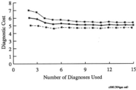
Fig. 3 shows the graphs for device c880. This device has 383 gates and 880 test points. As there are a large number of diagnoses, and only some of them are con sidered, different subsets. yield different results. Samples were gathered by randomly choosing different subsets of the diagnoses. The middle graph on the figure shows the mean, the upper and lower ones show one standard devi ation away. (These upper and lower curves are not used in this paper.) We have generated these curves for all of the devices in the test suite. These curves asymptotically approach log2n where n is the number of components in the device. This is roughly what one would expect in the situation where components have two fault modes and we only consider single faults. If there are n components, there are 2n initial diagnoses. On average, half of those are eliminated by the initial symptom leaving n possible diagnoses. Using binary tests to discriminate among n alternatives takes log2n probes on average. More gen erally, if components have f fault modes and the cardi nality of the diagnoses are l, we expect the diagnostic !.l!!i_ cost in these graphs to approach log2 2 . The shape of the curve is harder to estimate. The case where k < 3 (k is the number of diagnoses considered) is difficult to analyze. For k > 2, the result can be modeled fairly consistently with (cis diagnostic cost) a decreasing ex ponential:
Therefore the number of measurements saved by find ing one more diagnosis (beyond k) is:
There is one caveat worth mentioning in using this for mula: it makes the presupposition that the algorithmic strategy does not change for the duration of the session. In actual fact, the algorithm may increase or decrease k after subsequent probes. More likely it will decrease k because the value of higher k's drops as the number of diagnoses that remain drop. On the principle that the best prediction of a future decision is what we decide in the present, we use this formula.
4 Cost of Generating Another Candidate
The cost of generating another candidate is dependent on the kind of device, the size of the device, the inputs, etc. Again we are not able to come up with an ana lytic model of the computational cost of finding the next diagnosis. However, by observing the GDE/Sherlock al gorithm in operation one sees some valuable properties. Let's first look at the case where we are not making probes. GDE/Sherlock generates diagnoses at a roughly constant rate. Intuitively, one can see how this arises from the best-first search. During the best-first search most diagnoses are eliminated by existing conflicts. The best-first search avoids these diagnoses at nearly negligi ble cost. The significant cost is incurred when a candi date is discovered which is not subsumed by any known conflict, but we cannot be sure is free of conflicts. In this case we have to re-invoke the ATMS. If no incon sistency is found, then we have a new diagnosis. If an inconsistency is found, then a conflict(s) is found and used to accelerate the best-first search. Rarely does a device have a large number of conflicts worth recording before finding another diagnosis.
Therefore, our algorithm predicts the computational time to produce the next candidate as equal to the av erage time to find the candidates it has so far . In order to account for the rare case where the cost of generating candidates varies greatly, it includes the time spent since the last diagnosis was found in the calculation. There fore, if it spends a lot of computational effort to find the next diagnosis, then its prediction of when the next di agnosis will be found gets further and further out and if the time to find this diagnosis becomes too large the search is abandoned.
The introduction of probing has little effect on the rate of candidate diagnosis production. This can be qualitatively understood as follows. The addition of a probe makes the test of any candidate about twice as fast. This is partially due to the fact that a probe may have introduced new general conflicts therefore making it easy for the best-first search to skip these candidates directly. In addition, when a candidate diagnosis must be tested against the observations (at step 2), the TMS operations are faster because the probe fixed a device quantity thereby splitting the device and thereby short ening ATMS labels. As the probes tend to be quite good [8) even when k is small, the probe reduces the number of diagnoses by approximately ~. It reduces the number of diagnoses the algorithm has discovered by ~, as well as the yet undiscovered ones. Hence, discovering new diagnoses has become twice as difficult. The two effects tend to cancel yielding an unchanged rate of generation of new diagnoses. Table 1 illustrates the kind of costs we see in diagnosing devices.
| Candidate | Probe | .L\t(s) |
|---|---|---|
| 1 | 1 | .12 |
| 2 | 1 | .12 |
| 3 | 1 | .10 |
| 4 | 1 | .13 |
| 5 | 2 | .13 |
| 6 | 2 | .17 |
| 7 | 3 | .15 |
Although the rate of diagnosis production after a probe does not change, the number of diagnoses that remain to be found after a reasonable probe is halved. The probe has, in effect, eliminated these diagnoses for free.
5 A diagnostic algorithm which takes cost into account
In order to utilize our model our algorithm will always find at least (k = 3) candidates. This is both because our model of the benefit of a next diagnosis only applies if k > 2 and it allows for the computation a meaning ful average cost of diagnosis discovery. The algorithm is provided two exchange rates: ep which is the cost incurred per probe; e, which is the cost incurred per second of inference. The key step in the algorithm is to determine whether it is worthwhile to make another measurement. The implementation maintains a variable t (initially t = 0) which represents the time taken to find the current diagnoses. M will be the estimate of the number of probes necessary to isolate the diagnosis (log2 (!;)' initially).
- If they can be found before Sherlock's stopping cri teria is met, find 3 diagnoses which explain all the current symptoms. Update t with the time to find these diagnoses.
- If there is only one diagnosis , stop.
- If the stopping criteria has been met, go to Step 7.
- If M < log2 k, set M to log2k. Compute the benefit (B) of finding another candidate:
- If 1f- > B (i.e. , the cost of finding the next candi date outweighs the benefit) , then go to Step 7.
| e, | ep | GDE/Sherlock cost | New cost | p |
| 1 | 1000 | 5554 | 5554 | 5.6 |
| 1000 | 1 | 4705 | 3606 | 13.1 |
| e, | ep | GDE/Sherlock cost | New cost | p |
| 1 | 1000 | 2052 | 2052 | 2.05 |
| 1000 | 1 | 2904 | 966 | 2.3 |
- Allow the computation to run for Bk - t seconds e, or until another diagnosis is found . Update t. If a diagnosis is found, go to Step 3.
- Perform the probe (using one-step lookahead and then entropy) which best discriminates among the current k diagnoses. Divide M by 2.
- Remove the diagnoses eliminated by the probe re sult . Update k and t accordingly. Go to Step 1.
6 Experimental Results
We have run our algorithm on all the devices in our test suite. Table 2 lists the costs to diagnose a signifi cant sample of c880's faults. The first line in the table makes computation nearly free and probing expensive. This is the presumption of GDE's architecture and the resulting costs for GDE and the new algorithm are the same. In the second entry, cost of computation has be come extremely expensive. GDE which does not take cost of computation into account performs much worse, while the new algorithm performs significantly better. The last column of the table, p, is the average number of probes the new algorithm makes. Here we see the num ber of probes changes significantly depending on the cost tradeoff- exactly what one would expect. Table 3 shows the results for the smaller device C432 ( 432 test points, 160 components). The cost benefit of the new algorithm is clear for this device also.
7 Perspective from Decision Theory
Our algorithm can be viewed as a very simple, myopic, decision theoretic strategy. For clarity, the following analysis presumes binary valued variables. Let f(p, s) be our best estimate the cost to diagnose the device having made p probes and s candidates remaining. Our algo rithm repeatedly makes the decision of whether to probe or to compute. The decision of whether to compute or to probe is determined with one-step lookahead. The decision to probe has cost ep + f(p + 1, ~). The decision to compute is more complex to compute. We need to obtain the best estimate of cost if we continue to com pute. By tracking the costs to compute past candidates we maintain the mean and standard deviation of times to compute candidates. Let p(t) be the area under a normal curve from present to t. Suppose we compute for time t, the expected cost is:
We choose t such this is minimized.
For simplicity let us only compute changes of f(p, s) . Therefore, the cost of computation is the maximum of:
Our algorithm estimates f(p, s)- f(p, s + 1) directly (B in our algorithm). To accurately determine the cost of probing we need to compute f(p, s)- f(p + 1, ~) . We estimate this to be negligible as two effects tend to can cel. Every good probe reduces the number of possible candidates by ~ - Likewise every good probe reduces the number of known candidates by~ (i.e., the~) . Our pre liminary experiments demonstrate it to be of little utility to compute the standarq deviations and means of can didate computation costs . We will continue to use our simpler approximation for decision making. It is likely that if we encounter devices which have wide variance in candidate computation times that our approximation will become significantly suboptimal.
8 Summary
We have presented a simple algorithm which explicitly trades off computational cost against probing cost. By intermixing computation with probing, the new algo rithm lowers the total cost of finding a diagnosis over the less flexible approach that is usually employed.
The overall result is only a small beginning of the re search needed to understand the tradeoffs within diag nosis in order to develop minimal cost algorithms. There are a number of immediate simplifications made in this paper that need to be more closely analyzed. Some of them are:
- Our algorithm always needs at least 3 diagnoses to function. However, if probing is completely free there is no necessity to ever construct any diagnoses at all as the faulty component can be determined directly. Our algorithm's architecture does not ac commodate this possibility.
- Sometimes all faults of the initial cardinality are eliminated. Our algorithm needs to be extended to take this possibility into account.
- When the prior probabilities of component failure modes vary significantly, the estimate of the size of the diagnosis space (M) in the algorithm is too high, producing too high a benefit of future probes.
- The algorithm should be extended to accommodate varying probe costs. For example, it would expend a significant amount of computation, if the next probe to perform was very expensive.
- The model of the benefit of finding a new candidate was derived from the case where failure probabili ties are nearly equal and with the standard ultimate GDE/Sherlock stopping criteria (probability cliff) for finding new candidates. The stopping criteria used clearly influences the benefit of finding a next candidate.
- We observe that the algorithm usually lowers k dur ing a diagnostic session. Which is of little surprise as the number of diagnoses goes down, the advan tage of finding more candidates becomes less. How ever, our benefit model was based on a constant k. This probably introduces a small overestimation in the algorithms calculation of the benefit of a next candidate.
- We assume f(p, s)- f(p + 1, ~)is negligible. This needs more careful analysis and experimentation.
Acknowledgments
We thank Daniel Bobrow, David Heckerman and Eric Horvitz for their helpful comments and insights on this paper.
@inproceedings{ijcai1995p223,
  title     = {Trading off the Costs of Inference vs. Probing in Diagnosis},
  author    = {de Kleer, Johan and Raiman, Olivier},
  booktitle = {Proceedings of the Fourteenth International Joint Conference on
               Artificial Intelligence, {IJCAI-95}},
  publisher = {International Joint Conferences on Artificial Intelligence},
  editor    = {Chris S. Mellish},
  pages     = {1736--1740},
  year      = {1995},
  note      = {Qualitative Reasoning and Diagnosis},
  url       = {https://ijcai.org/proceedings/1995/223},
}
TY - CPAPER TI - Trading off the Costs of Inference vs. Probing in Diagnosis AU - de Kleer, Johan AU - Raiman, Olivier T2 - Proceedings of the Fourteenth International Joint Conference on Artificial Intelligence, IJCAI-95 PB - International Joint Conferences on Artificial Intelligence PY - 1995 SP - 1736 EP - 1740 UR - https://ijcai.org/proceedings/1995/223 ER -Copied
Machine-readable versions of this paper, for tools and AI agents:





