An Improved Constraint-Propagation Algorithm for Diagnosis

I Introduction

The diagnosis of a system exhibiting abnormal behavior con­ sists of identifying those subsystems whose abnormal behavior could produce the manifested behavior. In model-based diagnDsis, the system is treated as an idealized structure of components whose local behaviors interact to produce overall system behavior. Previous diagnostic schemes have tackled the task by partitioning the problem into two phases. First, making use of a set of observations and as­ suming the proper local behavior of components, predictions are generated about the behavior of unobserved points. In the second phase, the assumptions underlying those predictions contradi~ted. ~y observations are identified, and a set of hypotheses about the mdlVI­ dual component's behavior which "best" explains the manifested system behavior is assembled.

While many proposed schemes fit within this paradigm [Reiter 86, Genesereth 84), the work of [de Kleer et al., 1986) has especially focused on algorithms for performing these two ~ efficiently. In their scheme, predictions are generated by_ co~~t propagation [Stallman et al., 1977), while~ process of~dentifymg the (minimal) set(s) of assumptions underlymg a contradicted pred­ iction (confliCt sets) is facilitated by the ATMS machinery [de Kleer 86]. The diagnoses chosen as "best" are those minimal sets of as­ sumptions (candidates) which, if removed, render the model behavior compatible with the manifested behavior. 1bese are assem­ bled from the conflict sets by a set-covering algorithm.

*This work was supported in part by the National Science Foundation Grant DSR 83-13875.

associated with the values x 1 and x2 that variables X 1 aruf X 2 may take.

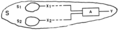
We can now consider the composite circuit fonned by an adder A with output Y and inputs X 1 and X 2· We are interested in finding the best labelings over the components of S compatible with the set of observations 0 = 0 1 u 0 2 and each of the possible values y of Y . In other words, we want to determine the labeling L (S ,0 u {Y = y }) for each value y of Y.

The main point to note is that, to detennine L (S ,0 u {Y = y }), we need not reconsider all the combinations of labelings over the individual circuits S 1 and S 2; L (S ,0 u {Y = y }) is made up of labelings that were already found optimal overS 1 and S 2 for some values of X 1 and X 2· In particular, assuming that the adder A is working properly (deooted by A = ok ), the weight associ­ ated with the optimal labeling will be given by:

where x 1 and x2 range over the possible values of X 1 and X 2, respec­ tively. Thus, if the minimum is achieved at values xi and xi, the optimal labeling for Y = y under the assumption A = ok, can be con­ structed from:

To find the overall optimal labeling, we must also include the possi­ bility that A is not working properly, denoted by A = -.ok, yielding:

The constant "1" stands for the penalty associated with component A being faulty, which in tum removes the constraint between the values of X 1 and X2. Notice that the tenns required to compute (1) and (3) depend only on the subcircuits S 1 and S 2, and were assumed to be available.

The overall best labeling(s) compatible with Y = y can now be obtained simply by comparing the weight computed from (1) with the one computed from (3) and choosing the labeling(s) correspond­ ing to the lowest one. If Y = y is now observed, L (S ,0 u {Y = y }) would emerge as the labeling defining the best diagnosis.

A question remains, however, of how to minimize over sets of values that, in principle, may have infinite cardinality. Its solution is based on the fact that there will be labelings which are compatible with all the values a variable can take. For example, in the simple adder circuit depicted in Figure 2, we have only two labelings, {A =ok} and {A =-.ok}. The best labeling compatible with X =6 is {A =ok} while, for any other value of X, {A =-.ok} is the best and, in fact, the only compatible labeling. Moreover, {A =-.ok} is the best labeling compatible with any value of X except X = 6. We will take advantage of this fact and will use the symbol nx as a place holder for all those, possible infinite, values of X which share the same optimallabelings. Referring to the example above, we will say that {A =-.ok} is the best labeling compatible with X =Ox. mean­ ing that it is the best (and probably only) labeling compatible with any value of X. The introduction of these "special" values will allow us to keep the state representation of the problem concise; the algo­ rithm, however, should behave as though an explicit representation were used for each possible value.

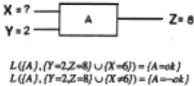
The example above illustrates two important properties on which our algorithm is based: first, that the problem of detennining the optimal labeling for a variable can be solved from infonnation associated with neighboring variables, ml!ldng feasible a distributed diagnostic inference engine in the fonn of constraint propagation; and secondly, that it is possible to incrementally predict all the possi­ ble model behaviors by encoding a finite (and usually small) set of "explanations," allowing the constraint propagation algorithm to ac­ complish the global identification task without appealing to non­ local set-covering procedures.

A critical assumption implicit in the example of Figure 1 is that circuits S 1 and S2 are only connected via A or, more generally, that the constraint netwo~ induced by the composite circuit S is singly-connected. In Section IV this assumption will be relaxed and we shall generalize the algorithm to deal with multiply-connected constraint networu. These extensions will provide interesting points of comparison with [de Kleer, 1986].

A. Notation

We assume that a component Ci can be in either of two states: it is wooong properly, denoted by cj =ok, or it is failing, denoted by Ci = -.ok. Since we are going to treat components as any other variable in the model, we will usually draw them as nodes as in Figure 3b. rather than depict them as blocks as in Figure 3a., where Ci e {ok,-.ok} stands for the name of the variable corresponding to the component status and j denotes the undirec­ tional constraint among the component input(s), its output(s) and its status.

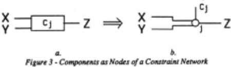
The resulting netwo~ is composed of

• nodes (or variables), denoted by upper-case letters (X, Y, W, ... , for observable system points and C;, Ci, ... ,for components);
• constraints, denoted by small letters (i , j, ... ); and

The set of nodes linked to a constraint k will be denoted by pic. A more useful set is P~ =Pic -X, which reads as the port k of node X, and stands for the set of all other nodes different than X linked to constraint k . C (X) will refer to the set of constraints linked to X . Lower-case letters x, y, w , ... ,ci, ci , ... ,will refer to the values of variables X, Y, W , ... , Ci, Ci, and subindices X I· X2, ... , wil be used to differentiate among the values of a single variable. We will extend this convention to refer to p~ as the values of the vari­ ables in the port P~. For example, the port Pj in Figure 3 is the set of variables {Y, Z, Ci}, while pj stands for their associated values {y, z, ci }. As stated before, the "value" Oy will serve as a place holder for all those values of node Y that are not explicitly represent­ ed.

In constraint-propagation algorithms such as the one used here, the ports of a variable contain enough information for the vari­ able to update its state. This updating is usually done incrementally, whenever a new state of a variable can be deduced from a neighbor constraint and its associated ports. We will use messages, denoted as m (P~ -+X), where node X is the recipient and port P~ the origin, to encode the intluence of the values of the variables in P~ upon X through the constraint k.

B. The Algorithm

Messages: Messages m(P~ -+X) are built from a vector of sub-messages m (P~ -+xi), where the xi's refer to values X may take. Each of these submessages is composed of three fields: xi, Nlc(xi) and Slc(xj), where the last parameter stands for the set of values p~ of P~ which would "best" support the potential observa­ tion X =xi and the second one for the weight associated with such support (i.e., the minimum number of faulty components, in the sub­ netwolk behind the port P~. necessary to account for X =x).

In short, a message m (P~ -+X) can be expressed as:

while each m (P~ -+xi) is a triplet :

If NJc(xi)=oo, for some value xi o(X, we simply remove xi from the set of values X that needs to be considered.

Message Combination: The first requirement for message combination is that every node save the last message received from each of its ports. New messages override old messages from any one port. From this set of messages, every node computes its state m (X). That is, if we denote the combination of messages by the symbol · n' then, for each of its values xi, X computes the states:

where

is called the weight associated with xi and represents the minimum number of faulty components necessary to account both for the current set of observations and the instantiation X =xi, and the support of xi, encodes the state(s) of the neighbomood of X that will best account for all the observations and the instantiation X =xi . Upon observing X =xi, the set of optimal diagnoses can be easily re­ trieved by tracing the support associated with xi. N (xi) represents the number of faults involved in any of these hypothetical diagnoses.

Message Assembling: Let port P~ contain the variables Y 1, Y 2, ... ,Y~. Then the parameters of the message m (P~ -+xi) are com­ puted from:

and

where the yj's range over the values of Yi· and Clc(Xi.YI.Y2· ... ,y~) denotes a predicate indicating the compatibility of its arguments ac­ cording to constraint k. The substraction of the component NJc(y) from the weight N (y) in (7) and (8) amounts to subtracting the con­ tribution to N(y) that originated in the port pic. This "orthogonaliza­ tion" is required to avoid counting the same fault more than once within a single diagnosis.

Initialization: The propagation algorithm requires that nodes be properly initialized. A node, C, representing a component status will be initialized to:

while any other variable Y will have an initial state:

Observations: The observation X =x is codified as a message from a virtual port Ox of X:

where absence of sub-messages corresponding to other values of X is interpreted as N (X =xi)= oo for any xi *x. For the purpose of ap­ plying formulas (5)-(8), for any observable node X, virtual ports Ox are taken to be members of the set C (X) of ports linked to X.

Control of the Propagation Process: While an orderly and incre­ mental propagation scheme would be the most efficient implementa­ tion in serial machines, the algorithm can also wolk under distribut­ ed control, in which each node inspects the state of its ports at its own discretion. The final state reached at equilibrium would be the same.

We now proceed to illustrate the wooong of the algorithm on a simple circuit discussed in [de Kleer 86], [Genesereth 84] and [Davis 84].

Ill Example

Let us consider the circuit depicted in Figure 4: Components M I· M 2 and M 3 are multipliers, while A 1 and A 2 are adders. The former will correspond to constraints C 1, C 2 and C 3, and the latter to constraints C 4 and C 5 · Initially, all inputs are known and propagated through the rest of the netwolk, generating the pattern of messages shown in Figure 5(a). Figure 5(b) displays the new states of nodes X and F.

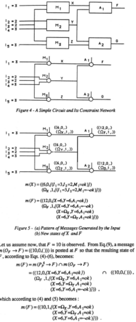
Since the value F = 10, has now three unit-weight supports, we can immediately assert that there are at least three different, equally mer­ itorious, diagnoses accounting for the enhanced set of observations, each of which is encumbered by a single faulty component (A 1, M 1 or M :z). We can uncover the identity of the faulty components in­ volved in these diagnoses by simply tracing their respective sup­ ports. For instance, underlying the support (X =Ox ,Y =6,A 1=ok) of F = 10, we find a single fault M 1 = -.ok associated, in tum, with the supportofX =Ox (Fig.5b).

The new message m ( 0 F -+ F) also causes a pattern of addi­ tiona! messages to propagate throughout the network. However, this propagation is necessary not for finding the diagnoses, (these can be found by tracing the existing supports) but for preparing the support lists of the network to accommooate new observations. Figure 6 il­ lustrates the computation of one of these messages, m (Px 4 -+X).

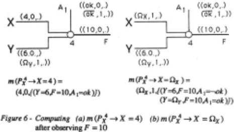
Note that, for the purpo~ of computing N 4 (X ), the weights associated with the variables in P.f (i.e., Y , F and A 1) do not include the contributions of messages originated from P 4 , as specified by Eq.(7). Figure 7(a) illustrates the new pattern of messages resulting after the observation F = 10. Each message is depicted next to its ori­ ginating port; additionally, any node that has received messages from more than one port computes its new state according to Eq.(4). Figure 7(b) displays the updated state of nodes A 1 and G.

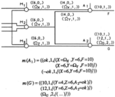
Let us assume now that G = 12 is observed. By simply trac­ ing the supports associated with this value of G , the optimal diag­ noses accounting for this and all previous observations is retrieved. Since the only support for G = 12 is (Y =6,Z =6,A 2=ok ), and the best support of Z=6 involves no fault, the two best explanations are found encoded in the support of Y=6, namely, either {M 1 =-.ok} or {A 1 =-.ok), respectively.

The computations required by the algorithm also provide useful infonnation for selecting points to test. Not only do the resulting data structures encode the best diagnoses accounting for any potential observation at any point in the circuit, but they also en­ code, through the supports attached to component nodes, the net­ worlc state most compatible with any component status. This turns out to be especially useful when we want to select test points to discriminate between different hypotheses.

Let us also note here that the scheme proposed does not guarantee finding all irredundant diagnoses [Peng 86], but only those with a minimum number of faults, i.e., the optimal diagnoses.

IV Enhancements

In this section we will discuss some modifications to the scheme introduced in Section II to enhance the types of models with which the algorithm can deal. We first discuss how to extend the message-passing algorithm to handle constraint networlcs containing loops and then propose a slight modification to accommodate models with specified component-failure probabilities.

A. Handling Constraint Networks with Loops

The strength of the proposed scheme lies in its ability to decompose global optimization problems into local ones. To achieve this, we assumed that messages received by a node from different ports carried independent infonnation, i.e., do not emanate from common observations. It is easy to find systems in which this as­ sumption is violated, as in the example of Figure 8.

z

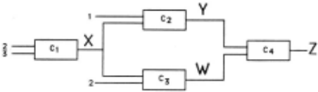
Clearly, the infonnation carried by both inputs of C 4 will depend on the status of C 1· Thus, knowing m(Y) and m(W) no longer suffices to compute m(Z). The reason is simply that, for some pairs of values y and w of Y and W, respectively, m (y) and m (w) might in­ volve a common set of faulty components; so, the weight associated with a value z of Z supported by y and w will not necessarily be the sum of the weights of its supporters. In addition, m (y) and m (w) may involve incompatible labelings of X ; so, we must ensure that they do not appear in a same support set.

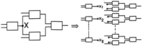
The solution that we will pursue is not new [Pearl 86.a] [Dechter & Pearl 86] and rests on the idea of treating a "loopy" net­ worlc as a family of singly-connected networlcs in which some of the variables (usually those corresponding to a cycle cutset and referred to here as "assumption" nodes) have been assigned a fixed value (Figure 9). A fixed-value node can be duplicated into a set of identi­ cal nodes, each connected to one and only one of its original ports while still preserving the overall behavior. To illustrate the modifications needed to handle loops, let us consider constraint net­ worlc S (Figure 10) in which the instantiation of assumption node A decomposes it into a pair of singly-connected networlcs, S 1 and S 2 . Let 0; denote the set of observations gathered in the subnetworlc S;. with i e {1,2} and let 0 =0 1 u02 represent the complete set of observations. Recalling the notation introduced in Section II, N (S ,0 ) stands for the number of faulty components needed to account for the set of observations 0 in system S. N (y) was then used as a shorthand for N (S ,0 u {Y =y }). We shall now use the abbrevia­ tions:

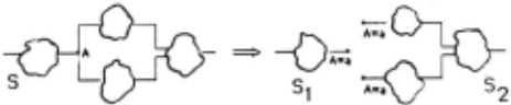
Notice that since the S; 's are singly-connected, the measure W 11 (x ), i.e. the minimum number of faults in S; , needed to account for the observations 0; u {A =a .X =x}, can be computed according to the procedure discussed above. We are interested, however, in computing the weight N(X=x)=N(S,O u{X=x}), i.e., the total number of faults in S needed to account for the entire set of observa­ tions 0 u {X =x} without any assumption about the value of A . This can be obtained by writing:

where

Thus, if the minimum is achieved at A =a ·, the optimal set of diag­ noses will be obtained from the supports associated with X =x under the assumption A =a · and from those associated with A =a · itself. From (10)-(14) it is clear that we will be able to compute N(y) for any node Y ,if we can compute W 11 (x) for every value a of A and every value x of the nodes X inS .

B. The Algorithm

and Each instantiation of the cutset variables identifies a set of singly-connected networks. We shall refer to the instantiated nodes as assumption nodes, to their instantiations as assumptions or tags, and to the states of the net compatible with a given set of assump­ tions as contexts. The manner in which tags are treated in this modified scheme bears a strong resemblance to the way assumptions are treated in the ATMS [de Kleer 86].

As with node values, the message-passing algorithm will not explicitely represent each of the possible values but will appeal, in­ stead, to the special 0-values introduced in Section ll. Now, howev­ er, tags containing n -values will be required to specify the range of values for which any n-value stands. For that purpose, we will use O(x 1, ... ,x,.) as the place holder for values of X other than x 1, ... , x,. . This will render a tag containing the instantiation X = x; incompati­ ble with any tag containing the instantiation X = O( ... .x; , ... ). The n-values assigned to non-assumption nodes are not required to keep this extra information explicit; so, for them, we use our previous, simpler notation.

Messages will now have the form :

where a represents the tag of the message, and each submessage rna (P~ -+ x) contains five fields:

where

w:(x) represents the component of Wa (x) originated in the k -th port of X;

s:(x) denotes its underlying suppon; and

N~(a) stands for the contribution Ni(a) to N(a), for XeS;. as received from the k -th port.

Note that N~(a) does not depend on the value of X. We have included it among the sub-messages in order to simplify the presentation.

The state of a node is computed by combining all messages with compatible tags received by the node from its different ports. For a value x of node X, the resulting state rn (x) is given by:

where Wa (x) and Sa (x) are computed as usual, within the context defined by each a, while the weight Nx (a) is computed from:

Messages are now assembled as in the case of singly­ connected networks, with the additional constraints imposed by the tags.

When a new observation, Y =y , is obtained, the optimal weight can be computed according to Eq.(l3):

where the weight N (a) is available at node A, and both Ny(a) and Wa (y) are available at Y. If Y e S;, and the minimum is achieved at A =a · , the set of optimal diagnoses can be obtained by tracing the supports Sa·(y) and [Si(a· )}, for j ;t:i . Additionally, the message posted by the observation Y =y will have the form:

where the last component amounts to setting N i (a) to the current value ofWa (y), as specified by Eqs.(lO) and (12).

Another problem generated by the presence of loops in con­ straint networks is the inability of unaided local constraint­ propagation methods to enumerate, in advance, all the distinguished instantiations of the cutset variables. For instance, if we regard t!le components in Figure 8 as adders, and we happen to observe Z=l3 instead of the predicted Z=l5, the only value of X compatible with C 1 = -.ok is X = 4. To arrive at this conclusion, we need either to solve a linear equation 2 ·X + 5 = 13 or to step sequentially through all the values in the domain of X. One way to obtain these solutions would be to permit the engine to propagate symbolic values [Stall­ man 77]. This approach seems suitable for implementation in the scheme proposed here and corresponds to viewing the n-values of assumption nodes as symbolic values.

For an illustration of how the proposed algorithm would handle the diagnosis of a circuit like the one depicted in Fig.8, the reader might refer to [Geffner et al. 1986].

C. Varying Failure Rates

The criterion of minimizing the number of faulty com­ ponents is reasonable in situations where there are no reasons to be­ lieve that different components fail with significantly different rates. If such is not the case, information about component failure rates could be easily integrated in the scheme proposed. One needs only to change the initial states of the component nodes. For example, in­ stead of initializing component node C;, to:

we can initialize it at:

where P; is the probability of failure in component C;, and k is any suitable constant.

For those cases (the majority) in which the components' failures are independent, the set of diagnoses obtained with this slight modification, will be those with the highest probability.

V Related Work

The diagnostic algorithm presented here grew out from the analysis and comparison of the scheme proposed in [de Kleer et al. 86] and the one reported in [Geffner et al. 87]. The former is a typi­ cal two stage algorithm. Predictions that assume the proper function­ ing of components whose failure was not established, are matched against the observations. A mismatch identifies a set of assumptions (conflicts) which cannot simultaneously hold. These sets are ob­ tained from the tags attached to the predictions refuted. From these sets, a non-local set-covering algorithm constructs the set of minimal diagnosis, i.e. minimal sets of violated assumptions which explain the observations.

1be diagnostic scheme reported in [Geffner et al. 87] is a probabilistic scheme in which both "right" and "wrong" behavior are considered on the same basis. Knowledge of the network topology (the singly-connectedness of the network is embedded in the algo­ rithm) and a set of probabilistic goodness measures attached to hy­ potheses, allow copious prunning, avoiding the combinatorial explo­ sion characteristic of unaided multi-hypothesis diagnostic algo­ rithms. On the other hand, the scheme seems unnecessarely expen­ sive for many applications, and it also requires the assessment of the probability distribution associated with the component's I/0 which, generally, is not available.

The scheme proposed here borrows from the latter what we consider to be its two main features : knowledge of the network to­ pology, and numeric qualification of candidate hypotheses. The algo­ rithm however can be interpreted as embedding two further assump­ tions : very small failure rates and uniform probability over the pos­ sible output values of failed components. The resulting diagnostic scheme can be thought then, as the non-probabilitic version of [Geffner et al. 87], in the sense that it can only accommodate a nar­ row set of probabilistic models. On the other hand, it only requires to propagate one type of message, it does not require the assessment of probabilities and it is sensibly less computationally expensive. Compared to [de Kleer et al. 86] and [Reiter 85], it does not require a non-local set covering procedure for identifying the culprits. More­ over in the singly-connected case, the knowledge of the network to­ pology permits to tag messages only with a numeric measure rather than with the identity of the assumption set. In the multiply­ connected case however, tags identifying the cutset assumptions are needed. In this respect, the scheme reported in [de Kleer et al. 86] which does not presuppose any knowledge about the type of net­ work, appears to be treating all variables as cutset variables. For sparse networks however, the preprocessing step needed to identify a cut set may be worthwhile.

VI Conclusions

We have introduced a distributed diagnostic algorithm which fully exploits the topology of the network of the system being diagnosed. The algorithm has linear complexity for singly-connected networks and a worst-case complexity of exp(l cycle-cutset I) for multiply-connected networks.

The proposed scheme departs from previous work by treat­ ing each component status as a variable, thus facilitating the predic­ ·tion of all possible model behaviors. This allows the message­ passing algorithm to perform the diagnostic task without appealing to non-local set-covering procedures. It also simplifies probabilistic approaches like [Pearl 86] by taking advantage of the deterministic nature of the models analyzed.

The intermediate computations generated by the algorithm provide information useful for the selection of new tests. Addition­ ally, information about component failure rates can easily be accom­ modated.