
Using Knowledge to Isolate Search in Route Finding
Proceedings of the Fourteenth International Joint Conference on Artificial Intelligence. Action and Perception. Pages 119-124.
© 1995 International Joint Conferences on Artificial Intelligence
Abstract
Traveling is a part of every person's day-to-day life. With the massive and complicated road network of a modem city (or country), fmding a good route to travel from one place to another is not a simple task. In Network Theory, this is the shortest path problem. Shortest path algorithms are often used to solve the problem. However, these algorithms are wasteful in terms of computation when applied to the route fmding task. They may also produce solutions that are not suitable for human drivers. In this paper, we present an approach that uses knowledge about the road network to substantially reduce the time and space required in computation, and to ensure human oriented solutions. Within this framework, three alternative methods are proposed, which may be used in different situations. A system has also been implemented for route fmding in Singapore.
- [Deo and Pang, 1984] N. Deo and C. Pang. Shortest path algoritluns: taxonomy and annotation. Networks, 14:257- 323, 1984.
- [Dial eta/., 1979] R. Dial, F. Glover, D. Karney, and D. Klingman. A computational analysis of alternative algoritluns and labeling techniques for fmding shortest path trees. Networks, 9:215-25, 1979.
- [Gallo, and Pallottino, 1986] G. Gallo, and S. Pallottino. Shortest path methods: a unified approach. Mathematical Programming Study, 26:38-64, 1986.
- [Goel eta/., 1991] A.K. Goel, T.J. Callantine, M. Shankar and B. Chandrasekaran. Representation, organization, and use of topographic models of physical spaces for route planning. In Proceedings of the 7th Conference on Artificial Intelligence for Applications (CAIA-91), pages 308-314, 1991.
- [Hayes-Roth et a/., 1983] E Hayes-Roth, D.A. Waterman, and D.B. Lenat (eds), Building Expert Systems, Addison- Wesley, 1983.
- [Helgason et a/., 1993] R.V. Helgason, J. L Kennington and B. D Stewart. The one-to-one shortest-path problems: an empirical analysis with the two-tree Dijkstra algoritlun. Computational Optimization and Applications, 1:45-75, 1993.
- [King and Mast, 1987] G. F King and T. M Mast. Excess travel: causes, extent, and consequences. Transportation Research Record, 1111:126-134, 1987.
- [Kuipers, 1978] B. Kuipers, Modeling spatial knowledge. Cognitive Science, 2(2):129-154, 1978. IJCAI
- [Levitt, and Lawton, 1990] T Levitt, and D. Lawton. Qualitative navigation for mobile robots. Artificial Intelligence, 44(3):305-360, 1990.
- [Lin eta/., 1994] Bing Lin, eta/. Finding the shortest route using cases, knowledge, and Dijkstra's algoritlun. IEEE Expert, 9(5):7-11, 1994.
- [Lin and Tay, 1995] Bing Lin and Jimmy Tay. Integrating knowledge-based and algoritlunic approaches for route finding. Forthcoming Report, 1995.
- [McDermott and Davis, 1984] D. McDermott and E. Davis. Planning routes through uncertain territory. Artificial Intelligence, 22:107-156, 1984
- [Pearl, 1988] J. Pearl. Heuristics. Addison-Wesley, Reading, MA, 1988.
- [Pohl, 1971] I. Pohl. Bi-directional search. Machine Intelligence, B Meltzer and D. Michie (eds), 6:127-140, 1971.
- [Sedgewick, 1988] R. Sedgewick. Algorithms, Addison- Wesley, 1988.
- [Shapiro et a/., 1992] J. Shapiro, J. Waxman, and D. Nir. Level graphs and approximate shortest path algoritlun. Networks, 22: 691-717, 1992.
- [Winston, 1992] P.H. Winston. Artificial Intelligence, Third Edition. Addison-Wesley, 1992.
References were extracted automatically from the PDF and may contain errors.
Full text extracted automatically from the PDF; figures, tables and equations may differ. The PDF is the version of record.
1. Introduction
One of the important computer applications in the transportation industry is route finding. Suppose we want to deliver some goods from our warehouse to a customer, we need to know the best route that will take us there. As another example, suppose a tourist rented a car and planned to drive around a city. He/she needs to know the way before going from one place to another. A computer route finding system will not only fmd the best route for the user, but also help to reduce the traffic in a road network. It is estimated that excess travel amounted 83.5 billion miles and 914,000 person-years annually at a total estimated cost of more than 4~ billion dollars per year in United States [King and Mast, 1987].
In Network Theory, route fmding is a shortest path problem [Deo and Pang, 1984; Dial et al., 1979]. Algorithms, such as Dijkstra algorithm [Deo and Pang, 1984] and A* [Pearl, 1988], are often used for solving this problem. However, these algorithms are general algorithms. They are wasteful in terms of computation when applied to the route fmding task. Most of the routes searched by the algorithms are actually irrelevant as they cannot possibly be part of the solution. Using only these algorithms may also produce solutions that are not suitable for human drivers. For example, human drivers would normally like to drive on major roads as far as possible, although using some minor roads may give the shortest path. In this paper, we propose a novel and yet simple approach of using knowledge about the road network to help a shortest path algorithm to perform the route finding task. It is termed as knowledge-based route finc:Iing. This approach dramatically reduces the time and space required in computation, and also produces human oriented solutions.
Although shortest path problem has been studied for decades, limited work has been done on using knowledge based technique to help solving the route fmding problem. We believe that one of the reasons is that Dijkstra algorithm, A* and others are already relatively efficient for the task. In the past, knowledge-based approach has been mostly applied for solving problems that do not have efficient algorithmic solutions [Hayes-Roth et al., 1983; Winston, 1992]. However, from our experiences, we can say that although Dijkstra algorithm (or A*) is efficient, knowledge-based approach can be successfully incorporated to produce even more efficient solution methods.
Our knowledge-based route fmding can be described as using knowledge about the road network to isolate the search and/or to guide the problem solving. Two key types of knot,\'ledge used in the proposed approach are the knowledge of road types (e.g., minor roads, major roads, and expressways) and the knowledge that major roads and expressways naturally partition the whole network into many small areas or sub-networks. These two types of knowledge and some others are used to partition and to reorganize the whole network. An efficient search algorithm is employed to search for the best solution in the appropriate sub-networks rather than the whole network. Within this framework, we present three specific methods. Each of these methods has its advantages and disadvantages over the others, and is suitable for a different situation. A system, called KB-RFinder, has also been implemented for route fmding in Singapore.
2. Shortest Path Algorithms and KnowledgeBased Method ·
Shortest path problem is modeled as fmding the shortest path between two nodes in a weighted and directed network G = (N, A) with a node setN and an arc setA. Each arc (i, J) E A also has a length (or weight) lij ~ 0. In the route finding context, the network is the road network. Nodes are road junctions, and arcs are road segments (a road may have a number of segments, however, below we will use roads and road segments interchangeably). The length of each arc could be the distance or the travel time between two adjacent junctions. The traveling direction allowed for a road segment corresponding to the direction of an arc.
Over the past three decades, many algorithms have been devised for the problem (see e.g., [Dial et al., 1979; Gallo, and Pallottino, 1986; Helgason et al., 1993]). Dijkstra algorithm is the classical algorithm for the problem. Most of the others are variations of Dijkstra algorithm. This algorithm can solve the problem in O((IAI + INI)logiNI) steps by using a binary heap [Sedgewick, 1988] for sparse networks (road networks are sparse networks). In our research, we have _ implemented many well-known algorithms, including Dijkstra algorithm [Gallo, and Pallottino, 1986; Sedgewick, 1988], S1 [Dial et al., 1979; Gallo, and Pallottino, 1986], S2 [Dial et al., 1979; Gallo, and Pallottino, 1986], and A* [Pearl, 1988], S12 [Helgason et al., 1993], S22 [Helgason et al., 1993], bi-directional A* [Pohl, 1971]. For road networks, A* is the most efficient algorithm. Interested reader, please see their performance comparisons in [Liu and Tay, 1995].
Although these algorithms are relatively efficient, applying them directly to route fmding is not appropriate. They are wasteful in terms of computation as in real situations it is not necessary to search through the whole network in order to fmd the solution. They may produce solutions unsuitable for human users as they may use too many minor roads, which is against the human preference of traveling on major roads.
Knowledge-based problem solving [Hayes-Roth et al., 1983; Winston, 1992] emphasizes the use of human problem solving strategies on a computer. This technology has been used in many applications.
However; for route fmding, using knowledge-based approach alone will not be efficient. Mter applying human knowledge about the network, a search is, still required to fmd the best solution. In most situations, knowledge is also unable to guarantee the best solution. It can only isolate the part of the network which could contain the solution, or prune off part of the network that is unlikely to contain the solution. Mter that, a search algorithm has to be used to find the best solution in the isolated area. In this case, A"' or (Dijkstra algorithm) comes to help.
From the above, it can be seen that each individual technique (algorithmic and knowledge-based method) does not provide a good solution method for route fmding. Each of them, however, does have its advantages in solving the problem. Analysis of their advantages and disadvantages shows that they can easily help each other. Thus, integrating them is the natural solution. We call this integration knowledge-based route fmding. We describe this approach in the next 4 sections
3. Knowledge About the Road Network
Before presenting our approach, we first describe the key types of knowledge we use. There are two main types:
Road types: Typically, in a city road network, there are three types of roads, minor roads, major roads and expressways. Knowledge about road types is crucial in route fmding for two reasons. Firstly, people prefer to drive on expressways and major roads. A practical system should meet this preference. Secondly, road type knowledge also help to prune the search space in problem solving as we will see later.
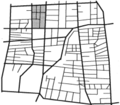
Major roads partition the whole road network: When we look at the road map of a city, an important feature that can be observed is that major roads and expressways themselves also form a network (we call it the major road network or MRN for short). Expressways may not form a connected network in a city, but may form a network in a state or country. We group major roads and expressways into one class and call them major roads because expressways normally make up only a small part of the road network in a city, which is our primary concern. However, our ideas developed subsequently can be generalized to expressways for inter-city and inter-state route finding. Figure I (major roads are in thick lines and minor roads are in thin lines) shows a small part of the Singapore road network.
We can further observe from the map that MRN naturally partitions the whole network into many smaller areas (or sub-networks) (see Figure 1). The shaded area is an example. This is the key idea of our approach, which uses this natural partition to isolate the search.
4. Using Knowledge to Isolate Search
The ideal situation in route fmding, particularly for a long distance travel, is as follows: Assume that a driver plans to go from one location (the source S) on a minor road to another location (the destination D) on another minor road. Ideally, the route fmding system should search in a small area around S to reach some major roads (to reach the nearest major road may not be sufficient, we will elaborate on this in Section 8). Within this area, it will consider both major and minor roads. After this, it should consider only major roads. When it is approaching D, the system again should search in a small area in which both major and minor roads are considered in order to reach the destination. Figure 2 illustrates this scenario. Grids are used to show the isolated areas. This approach has two advantages: (1) it prunes off a great deal of search space; and (2) it produces routes that satisfy people's preference of traveling on major roads.
Obviously, this ideal case does not guarantee the best solution. But, the solution may be good enough as people do prefer to drive on major roads. In real life, we do not always ask for the best solution. A good solution will be sufficient. Now, the problem is how to form these grids. We discuss our approach to this below.
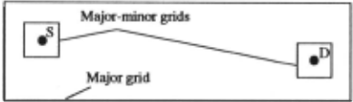
In the new technique, we will not form the major grid as in Figure 2, i.e., all the major roads are considered. When A* is used instead of Dijkstra algorithm, it automatically searches in the direction of the destination. Thus, only the two major-minor grids need to be formed.
In Section 3, it was noted that MRN naturally partitions the whole network into many small areas. All the minor roads in each area can be accessed from the major roads around them. Hence, we can statically assign each node (or junction) in the small area that area as its grid. Thus, in the proposed approach, a road network is represented as a major road network and many small sub-networks (each grid represents a sub-network). Within this framework, three specific network representations and their respective problem solving methods will be discussed. They are the topics of the next two sections. Here, we shall focus on the grid formation, which is a process of partitioning the road network into many small grid sub-networks. The important cases are as follows:
- Major roads surrounding a set of minor roads naturally form a grid sub-network for every node (or junction) in the minor roads. The shaded area in Figure 1 shows such a grid sub-network. The minor roads inside the grid are connected, i.e., they are connected without considering their traveling directions allowed.
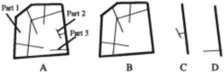
- Although major roads naturally form many grid sub networks, the minor roads in a grid sub-network may not be connected among themselves. For example, Figure 3(A) shows a natural grid sub-network that has three unconnected parts (only connected via major roads). It is obvious that traveling to or from any node in one part will not need to pass the minor roads in any other part unless the source or the destination is in that part. Hence, three smaller grids may be formed (see B, C and D in Figure 3). This separation further reduces the search. Notice that each smaller grid sub-network contains the major roads around it. This is to facilitate the linking up operation when we need to link a grid sub-network to MRN. Notice also that a grid may not need major roads to surround it (see C and D of Figure 3).
The above grid formation could be done automatically. It appears that quite amount of processing is needed. This is not a problem. It is important to recognize that this only needs to be done once. Once constructed, it is used again and again to fmd the shortest route for any problem.
5. Representing the Road Network
From the last two sections, two key concepts have emerged, namely, MRN, and grid sub-networks. They together represent a complete network. Here, we presents three alternative methods for representing and storing a road network. Their respective problem solving methods are presented in the next section.
Method 1. In this first method, the whole network is represented as many pieces, a major road network and many grid sub-networks. The required grid sub-networks are linked to the major road network when needed in route fmding. The actual implementation can be in various forms. The important thing is that each grid sub network should be indexed so that it can be retrieved in constant time when needed. This method does not save space because everything is still in the system.
Method 2. Like method 1, the whole network is also represented as many pieces. However, only MRN is permanently in the system memory, while all the grid sub-networks are stored in a hard disk or a CD ROM. Each of them could be in an indexed file such that it can be loaded quickly. When a query requires a node (either the source or the destination) in a grid sub-network, that sub-network will be read in. This method requires very little system memory because normally a large majority of roads are minor roads.
Method 3. This method represents the whole network as one piece just like that for Dijkstra algorithm. However, each node in a gird is marked with its grid number. A node that is on a minor and also a major road is considered as a major road node. All the major road nodes are marked with 0. Like method 1, this method does not save space as everything is in the memory.
6. Problem Solving Algorithms
This section presents the problem solving algorithms for the above three network representations respectively.
Method 1. The algorithm for this method is given below.
Step 1. H the source is a node on MRN then go to Step 2
else (1). retrieve the grid for the source
(2). link the gird sub-network to MRN Step 2. H the destination is a node on MRN then go to Step 3
else H the destination is in the same gird as the
source then
go to Step 3
else (1). retrieve the grid sub-network for the destination
- (2).link the sub-network to MRN.
Step 3. Run the shortest path algorithm (e.g., A* or Dijkstra algorithm) with the augmented MRN.
Step 4. Remove the sub-networks added into MRN.
Let us analyze the complexity of this algorithm. (1) in Step 1 and 2 can both be done in constant time as each node can be associated with its grid sub-network. Linking each grid sub-network to MRN in (2) of Step 1 or Step 2 is only linear to the number of major network nodes that surround the grid. The computation required is very small and negligible. Implementation details of this link-up operation can be found in [Liu and Tay, 1995]. Step 4 is also negligible. So, the main computation comes from the shortest path algorithm (e.g., A*). Because the number of nodes and arcs have been substantially reduced, it will run much faster than with the complete network.
Method 2. The algorithm for this method is almost the same as that for method 1 above. The main difference is that ~ Step 1(1) and Step 2(1). the appropriate sub networks are loaded in from a hard disk or a CD ROM. The link-up operation is also done differently from method 1 because the sub-networks need to be formed frrst before they are linked to MRN.
Method 3. This method is simple. A* (or Dijkstra algorithm) can be modified so that before visiting a node it checks to see whether the node is in the source grid, or the destination grid, or on a major road. If it is, it will be considered. Otherwise, it will be dropped. It is clear, the complexity of this method is the same as A* (or Dijkstra algorithm).
This method has an interesting property. Note that using grid sub-networks and MRN in method 1 and method 2 creates a problem where some shortcuts by using minor roads could not be considered such that the solution found may not be the shortest. For example (see Figure 4), we are traveling from 1 to D, assuming D is in a grid sub network and 1 is an intermediate node on MRN (the source is far away). Using method 1 and 2, only minor roads in the grid sub-network where D is located will be considered. The minor road 2-5 will not be in. In this case, the path will be 1-2-3-4-5-D. Obviously, this is not the shortest path if 2-5 is included. The path 1-2-5-D is defmitely shorter in terms of distance (assuming it is also true of traveling time). 2-5 is a shortcut.
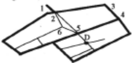
Method 3 is able to handle this type of simple shortcuts. In the 1,1bove example, when the system searches the nodes from 2, the road segment 2-5 will be considered because node 5 is on a major road. This method, however, cannot consider shortcuts that have more than one segment between two nodes on major roads, e.g., 2-6-5.
Although this method is only able to handle one-segment shortcuts, surprisingly the results listed in the next section show it can produce solutions that are very close to optimal ones using the Singapore road network.
All the above discussion follows the ideal situation in Section 4, which is for long distance travels. So how about short.and medium distance travels? Indeed, it is easy to see that they can also use the proposed techniques.
7. Evaluations
The aim of this project is to build a road guidance system for cars and other types of vehicles in Singapore. A prototype, called KB-RFinder, has been implemented. It is based on method 1 above with A* as its search algorithm. It uses the whole Singapore road network, which has over 12600 nodes and 30700 road segments. Out of this, about 1100 nodes are major road junctions forming MRN. The number of grids formed is 958.
The system is implemented inC on a 486 PC. Due to the space limitation, we are not able to describe the system in detail. Interested reader, please refer to [Liu and Tay, 1995]. Here, we concentrate on the evaluation of the proposed techniques.
We have implemented all the three methods. The second method was implemented by storing the grid sub-networks in the hard disk of our PC. So far, numerous tests have also been performed, using short, medium and long distance travels. The results from method 1, 2 and 3 are compared with those obtained by using the full network, i.e., without any grid (we call this method method 0). Both Dijkstra algorithm and A* are employed as the search algorithms for comparison.
Two sets of results are given below. One set uses travel distance as the cost function, and the other uses travel time as the cost function. Each algorithm solves 100 problems for every distance category using the same randomly generated sources and destinations. The running time (in second) is the sum of times in solving the 100 problems. Travel distance (in meter) and travel time (in minute) are the sum of distances and the sum of times of the 100 problems respectively.
| Number of problems= 100 | Cost: minimal travel distance Dijkstra A• | |||
|---|---|---|---|---|
| Running | Running | Travel | ||
| Category | Interval(km) | time(sec.) | time(sec.) | dist.(m) |
| Using full network (method 0) | ||||
| short | [0, 15) | 9.40 | 3.27 | 563404 |
| medium | [15, 30) | · 32.39 | 14.42 | 1951254 |
| long | [30, inf) | 40.00 | 27.88 | 3019790 |
| Using grid sub-networks (method 1) | ||||
| short | [0, 15) | 1.48 | 0.85 | 608120 |
| medium | [15, 30) | 3.50 | 1.70 | 2169321 |
| long | [30, inf) | 3.26 | 3.40 | 3443898 |
| Using memory and disk (method 2) | ||||
| short | [0, 15) | 24.91 | 24.46 | 608120 |
| medium | [15, 30) | 20.61 | 19.52 | 2169321 |
| long | [30, inf) . | 19.06 | 18.25 | 3443898 |
| Using node testing (method 3) | ||||
| short | [0, 15) | 3.21 | 1.71 | 593563 |
| medium | [15, 30) | 8.64 | 4.20 | 1996958 |
| long | [30, inf) | 10.16 | 7.82 | 3098761 |
From the above table, we can see that when using travel distance as the cost function method 1 improves the performance by 7-9 times (comparing with Dijkstra algorithm and A* using the full network), and method 3
improves the performance by 3-4 times. As expected, method 1 outperfonns method 3 significantly as method 3 needs to test each node along the search.
Regarding the travel distance, method 1 and 2 produce routes arou~d 9% longer than the optimal routes. Although method 3 ts only able to handle simple shortcuts, it produces routes that are very close to the optimal solutions.
When using travel time as the cost function (see the table below), the running time comparison of various methods still apply. For the travel time, method 1 and 2 also produce routes that take around 9% more time than the optimal routes. Again, method 3 produces routes that are very close to the optimal solutions.
| Number of problems= 100 | Cost: minimal travel time Dijkstra | |||
|---|---|---|---|---|
| Category | Running | A* Running | Travel time(min) | |
| Interval(km) time(sec.) time(sec.) Using full network (method 0) | ||||
| short | [0, 15) | 9.54 | 6.01 | 689.78 |
| medium | [15, 30) | 33.31 | 25.43 | 2250.81 |
| long | [30, inf) | 42.36 | 40.97 | 3512.61 |
| Using grid sub-networks (method 1) | ||||
| short | [0, 15) | 1.30 | 1.07 | 726.94 |
| medium | [15, 30) | 3.50 | 1.92 | 2475.64 |
| long | [30, int) | 3.88 | 3.38 | 3903.72 |
| Using memory and disk (method 2) | ||||
| short | [0, 15) | 23.29 | 22.85 | 726.94 |
| medium | [15, 30) | 20.23 | 19.58 | 2475.64 |
| long | [30, inf) | 19.60 | 19.56 | 3903.72 |
| Using node testing (method 3) | ||||
| short | [0, 15) | 3.39 | 2.21 | 706.85 |
| medium | [15, 30) | 8.31 | 6.94 | 2259.01 |
| long | [30, inf) | 9.89 | 9.56 | 3517.76 |
For all our tests, we did not consider the waiting time, starting and slowing down time at traffic lights. When these are considered, we believe all the methods will be able to produce results that are much closer to the optimal solutions because the new methods travel mostly on major roads and expressways, which have less or no traffic lights.
The running time performance of the second method cannot be compared with the other two in both cases since disk accesses are involved in loading in sub-networks. However, it is more efficient than method 0 for medium and long distance travels. It can also be noted that the running times for different distance categories are not that different. This is because the disk access dominates the c.omputation in this method. It is also seen that running ttme for long distance travels is slightly shorter than for short distance travels. This is because for short distance travels many grids could be in the city centre areas, where a grid tends to have more minor roads in it than the outskirts of the city. For long distance travels, the grids are mainly in the outskirts of the city.
Let us now discuss in what situations each of these three methods should be applied.
- The first method and the third method can be used in situations where the whole network can be loaded into the system. Method 3 is much easier to implement and
also produces routes that are very close to optimal solutions (although it is not as efficient as method 1). It may be used in the situations where its performance is acceptable. The first method is more difficult to implement because of its complex network representation and linking up opemtions. However, it is much more efficient than method 3. Both these two methods do not save any memory space.
- The second method should be used in situations where storing the whole network in the system is not possible. For a 486 PC with 4MB of RAM, the largest network that can be used is 13000 nodes and 50000 arcs without road names loaded in. If we have the road network of a state or a country and still use a small machine such as a PC or an even smaller specific system, a large part of the road network (or the whole network) has to be stored in a hard disk or a CD ROM. In these cases, our approach of partitioning, reorganizing and storing the road network as many pieces becomes valuable as it allows minimal data to be retrieved for route finding.
8. Related Work
Shortest path problem has been studied extensively in Network Theory over the past three decades. Many efficient algorithms have been produced [e.g., Dial et a/., 1979; Gallo, and Pallottino, 1986; Pearl, 1988]. However, limited research has been done in adapting these algorithms for route finding purposes. In AI, a number of studies have also been made. Their emphasis has been on using topographic and geographic knowledge and reasoning to solve the problem [Kuipers, 1978; Levitt, and Lawton, 1990; McDermott and Davis, 1984; Goel eta/., 1991]. The major concerns in AI are spatial knowledge representation and reasoning, mther than efficiency and optimization.
[Shapiro eta/., 1992], which is the latest work we could fmd in network theory and its applications, propose a technique to use level structure of the road network to help searching for a path efficiently. Applying their technique to our problem, it will be like this. Assuming the source and the destination are both on some minor roads. The algorithm will first search for the nearest entry point u to and the departure point v from MRN from the source and the destination respectively. After that, it uses Dijkstra algorithm to search only the major roads to fmd a path linking u and v. This technique indeed minimizes the time traveling on minor roads and also greatly reduces the search. However, the problem is that the two nodes u and v connecting the source and the destination to MRN could be on the wrong major roads. Then, the path found would be quite far from the shortest path. This technique is particularly not good for short and medium distance travels.
Our approach solves this problem by using grid sub networks. This means there will be no problem of landing on the wrong major roads because all the major roads surrounding the source or the destination are considered.
Our approach also offers a way to partition the whole network into small sub-networks that can be stored sepamtely. This will be important for large networks.
The work reported in this paper is a continuation of our earlier R-Finder system [Liu et a/., 1994], which uses Dijkstra algoritlun, knowledge-based technique and case based reasoning for route finding. KB-RFinder has made many improvements over R-Finder. The most important improvement is on the grid formation. In R-Finder grids are assigned at run time for each problem, rather than formed statically for each node as in KB-RFinder.
Each grid used in R-Finder is a rectangle that encloses a small area of the network. Figure 2 actually shows such an example. The sizes of the grids around the source and the destination are decided according to the density of the road network at their respective locations. For a dense part of the road network, the grid is smaller and for a sparse part of the network, the grid is bigger. The major grid (see also Figure 2) is determined according to the major roads between the source and the destination. This approach has a number of problems:
- The network knowledge used only provides qualitative information. There is no quantitative guideline. It is still difficult to decide precisely how big a grid should be and where the grid should be.
- It can also be seen that this approach requires a great deal of network and geographical knowledge. Then, knowledge representation presents a difficult problem.
- The system built with this method may be useful only in a particular place due to the heavy use of local network knowledge. It is useless in another place as the road network of the place will be completely different.
It is these difficult issues that have prompted us to seek a better solution. In KB-RFinder, all the above problems with the dynamically assignment of grids are eliminated.
- Firstly, in static formation of grid sub-networks, there is no such problem of deciding the shape and the size of each grid. A gird is simply a sub-network.
- Secondly, there is no need to acquire a large amount of network knowledge and to have a complicated knowledge representation. Although static formation of grids also requires various types of knowledge, as we can see they are very simple.
- Thirdly, this technique can be easily applied to build systems in other places since the types of knowledge used are generic to most modem road networks.
The performance of KB-RFinder is also much better than R-Finder. R-Finder typically uses half of the time taken by a pure Dijkstra algoritlun without any grids, while KB RFinder uses only around one eighth of the time.
9. Conclusion
This paper presented a novel and yet simple approach and three specific methods for practical route fmding. They exploits two key kinds of knowledge about a road network, namely, road types and the fact that major roads naturally partition the whole network into many small sub-networks. These kinds of knowledge help to reduce the computation time and space required for route fmding considerably. They also guarantees human oriented solutions.
The proposed approach and its specific methods are general as the types of knowledge they use are very simple and generic to different road networks. They can be readily applied to build route fmding systems in other places.
Acknowledgments: I would like to thank Land System Support Unit, Ministry of Law, Republic of Singapore for providing Singapore road network data. Without it, this project would be impossible. I would also like to thank Jimmy Tay, Hui-Peng Gob, Mary Heng, and Sook-Ming Hong for implementing various parts of the system.
@inproceedings{ijcai1995p16,
  title     = {Using Knowledge to Isolate Search in Route Finding},
  author    = {Liu, Bing},
  booktitle = {Proceedings of the Fourteenth International Joint Conference on
               Artificial Intelligence, {IJCAI-95}},
  publisher = {International Joint Conferences on Artificial Intelligence},
  editor    = {Chris S. Mellish},
  pages     = {119--124},
  year      = {1995},
  note      = {Action and Perception},
  url       = {https://ijcai.org/proceedings/1995/16},
}
TY - CPAPER TI - Using Knowledge to Isolate Search in Route Finding AU - Liu, Bing T2 - Proceedings of the Fourteenth International Joint Conference on Artificial Intelligence, IJCAI-95 PB - International Joint Conferences on Artificial Intelligence PY - 1995 SP - 119 EP - 124 UR - https://ijcai.org/proceedings/1995/16 ER -Copied
Machine-readable versions of this paper, for tools and AI agents:





