Dynamic Trajectory Planning Path-Velocity Decomposition and Adjacent Paths

1 Introduction

1.1 The Problem

Ever since Nilsson 's work in 1969 [Nilsson, 19()9), Mo­ tion Planning has been extensively studied (the reader is referred to [Latombe, 1990) for a recent. survey of this topic). Previous works can be classified according to the type of motions which are planned; it. is possible t.o dif­ ferentiate between Path Planning which is characteri~ed by the search of a continuous sequence of configurat.ions, 1 and Tr·ajectory Planntng which is concerned with t.he time history of such a. sequence.

Path Planning is restricted t.o the geomet.ric aspects of l'vlotion Planning. The only constraints which can be dealt with are time-independent. constraints such as stationary obstacles and kiuematic constraints, i.e. con­ straint.s involving the configuration parameters of t.he robot and their derivatives. Depending on whether it. is ho/onom.ic or not.~ a kinematic constraint either reduces the set of allowed configurations or restricts the geometric shape of feasible paths (see [Barraquand and Latombe, 1990) for more details) . On the other hand, Trajectory Planning permits to take into account time­ dependent constraints such as moving obstacles and dy­ namic constramts, i.e. constraints on the forces or the accelerations applied to the robot.

·This work wa$ supported h~· t.he French l'vlinist.ry of Research and Space and the Europe;w EUREKA projet. PROMETHEUS Pro-Art.

1 The configumtiou of a robot. is a set. of independent pa­ rameters of minimal cardinality which uniquely define!:< the position and orientation of every point. of the robot..

2 A kinematic constraint. is holonomic if it. is integrable,

"Vhen planning the motion of an actual robot , it is important to take into account the various constraints which restrict. its motion capabilities. It is also important t.o deal with moving ob::>tacles ,,ince an actual workspace will often be dynamic, i.e. with moving obstacles. These points have been addressed in the past, but, as far as we know , never simultaneously~and it is our goal to try to do so. Thus, in this paper. we will study Dynamic Trajectory Planning which is defined as Trajectory Planning for a robot. moving in a dynamic workspace. Besides the kinematic and dynamic const raints of the robot will be taken into account.

1.2 The Approach

We consider the case of a car-like robot A with bounded velocity and acceleration, moving in a dynamic planar workspace W. Note that, because it is a wheeled robot , A is subject to non-holonomic constraints (see §3.1 ).

There are no complexity results for the two­ dimensional instance of Dynamic Trajectory Planning that we consider. However results about similar prob­ lems suggest that it. is intractable ( cf. the NP-hard result established in [Canny, HJ88) and the P-Space algorithm presented in [Canny et a/., 1990)) . On the other hand, the one-dimensional case seems less intricate ( cf. the polynomial algorithm presented in [O'Dunlaing, 1987)). These results motivated us to use Path-Velocity Decom­ position [Kant and Zucker, 1986) which address~s Motion Planning in two complementary stages: (a) planning a geometric path which avoids the stationary obstacles and (b) planning the velocity along this path so as to avoid the moving obstacles . This approach is of a practical interest. because it. clc>composes the original problem into two more simple problems. However it presents a serious drawback: it cannot find a solution if a moving obstacle stops right on the computed path. The usual answer to this problem is to consider a set of candidate paths [Pan and Luo, 1990]. Our own answer is the novel concept of adjacent paths. Adjacent paths will be formally de­ fined in §5. Meanwhile, an informal illustration of what adjacent paths are can be found in the roadway: roads are usually divided into several adjacent lanes and every driver knows what passing from one lane to an adjacent one means.

i.e. if the derivative of the configuration parameters can be eliminated.

3 Except in [Fujimura and Samet, 1989) and [O'Dtlnlaing, 1987) but. with simplifying assumptions.

Thanks to this concept, we have designed a novel mo­ tion planning schema which operates in two complemen­ tary stages . The first stage, Paths Planning, takes into account all the time-independent features of the problem at hand (stationary obstacles and A's kinematic con­ straints) whereas the second stage, Trajectory Plan­ ning, deals with the time-dependent ones (moving ob­ stacles and A's dynamic constraints) . In Paths Plan­ ning, a set. of adjacent pat.hs, one of which leading A to its goal, are computed. These paths are collision-free with the stationary obstacles and respect A's kinematic constraints. In Trajectory Planning, knowing t.hat A is able to shift. from one path to a.n adjacent. one freely, we determine the motion of A along and between these paths so as to avoid any collision with the moving ob­ stacles while respecting A 's dynamic const.raint.s.

1.3 Content of the Paper

§2 reviews the works relat ed t.o Dynamic Trajectory Planning. Then §3 formally states the problem at. hand. Afterwards §4 describes an algorithm which solves this problem by using Path-Velocity Decomposition while ~j5 presents the concept. of adjacent. paths and shows how it. can be used to extend the previous algorithm. Finally experimental results are presented in §6 .

2 Related Works

To our knowledge. [Fujirnura. and Samet.. 1989] and [O'Dt'mlaing, 1987] are the only references address­ ing Dynamic Trajectory Planning but. with far t.oo sim­ plifying assumptions. On t.he other hand, there are nu­ merous works which are of a particular int.erest. t.o our problem. The works addressing either tnoving obstacles. non-holonomic kinematic constraints, or dynamic con­ straints are reviewed in the next. three :wctions.

2.1 Moving Obstacles

The general approach which deals with moving obstacles is the 'configuration-time space' approach: it. consists in adding the time dimension to the robot. 's configura­ tion space. Accordingly the different. approaches devel­ oped in order to solve the path planning problem in the configuration space can be used (cf. [Lat.ombe, H.J~10]). Among the various existing works, we can dist. in~uish those based upon extension of t.he visibility graph lErd­ mann and Lozano-Perez. 1986] and those based upon cell decomposition [Shih et a./., 1990] {[Fujimura. and Samet, 1989] falls into this latt.er category).

2.2 Non-Holouomic Constraints

As for car-like robots, Laumond [1 986] was the first to give the condition of existence of a feasible path. He shows that if some path exists then it is always possible to transform it into a feasible path . In the wake of this result , several authors [Jacobs et a/., 1991 ; Jacobs et a/., 1990; Jiang et a/., 1992] have proposed path planners which operate in two steps: {a) a path disregarding the non-holonomic constraints is computed and (b) this path is turned into a feasible path . Other approaches are presented in [Barraquand and Latombe, 1989] and [Tournassoud and Jehl, 1988] . Furthermore several authors [Jacobs and Canny, 1989; Laumond, 1987; Wilfong, 1988] have studied the problem of plan­ ning a path without. manreuvres, i.e. without inversion of the direction of motion; this problem appears to be more difficult . The crucial fact. about all these methods 4 is that they generate paths made up of straight seg­ ments connected with tangential circular arcs of mini­ mum radius (such paths are the shortest ones for car-like robots [Dubins, 1957; Reeds and Shepp , 1990]).

2.3 Dynamic Constraints

There are results for exact time-optimal trajectory planning for Cartesian robots subject. to bounds on their velocity and acceleration [Canny et a/. , 1990; O'Dunlaing, 1987]. Besides optimal-control theory pro­ vides exact results in the case of robots with full dy­ namics moving along a given path [Bobrow et a/. , 1985; Shin and l\1cKay, 1985] . However the difficulty of the general problem and the need for practical algorithms led some authors to develop approximate methods. Their basic principle is to define a grid which is searched in order to find a near-optimal solution. Such grids are defined either in the workspace [Shiller and Dubowsky, 1988]. the configuration space [Sa.har and Hollerbach, 1985]. or the state space of the robot [Jacobs et al., 1989; Xavier, 1 992] .

3 Statement of the Problem

3.1 The Robot A

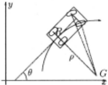
Let A be a car-like robot, it ha.c; two rear wheels and two directional front. wheels . It is modelled as a poly­ gon moving on IR 2 . A configuration of A is completely defined by the 3-t.uple (x,y,B)EIR 2 x(0,27T( where (x,y) are the coordinates of the rear axle midpoint R, and () the orientation of A {Fig.1 ).

4 Except. [Jacobs et al., 1991].

3.1.1 Kinematic Constraints

A body moving on the plane has only one centre of rotation . Let G be A's center of rotation . Assuming pure rolling condition, a wheel can only move in a di­ rection which is normal to its axle. Therefore, when A is moving, the axles of its wheels intersect. at. G. The orientation of the rear wheels being fixed , G is located on the rear wheels axle (possibly a.t a.n infinite distance) and R moves in a. direction which is normal to this axle. In other words, the following constraint holds :

Besides, due to the fact. that the front wheels OI'ien­ ta.tion is mechanically limited , the distance p between Rand G, i.e. the curvature radius at point R, is lower bounded , namely :

Relations (1) and (L) are non-holonomic. As wP will see further down , they restrict. t.he geometr ic shape of feasible paths for A .

3.1.2 Dynamic Constraints

Let. v be the velocity of A measured a long its main axis and let. O.r.a n and a.,..,d be respectively the tangential and radial components of the acceleration app li ed to A. The following dynami c constraints should lw sat isfied:

The meaning of these constraints is quite straightfor­ ward. Inequality (3) is a simple speed limit and (4) is an upper bound on the rate of change of speed. The purpose of (5) is to ensure that. the radi al accelerill.ion does not exceed the counterac ting centrifuga l accelera­ tion which is supplied by friction between the wheels and the ground. Although simple, these dynamics con­ straints are rich enough to demonstrate the i nt.erest. of our approach. More accurate dvn amics constraints could easily be dealt with (d'. [Fra icl;ard, HJ~l3]).

3.2 The Workspace W

W = IR" , it is cluttered up with stationa ry obstac les Bt, i = 1. .. s, and \\'it.h moving obstacles BjH, j = 1. .. m . Both types of obstacles are modelled as convex polygona l regions of W .

3.3 The Solution

In this framework , a t.raject.ory he tween a 11 in i t.ial con­ figuration q, and a fin a l configuration q,. 1 is defin ed by a mapping f taking a t.inw IE[O, I r J t.o a configura­ tion f(t) = (a:(t) , y(t) , B(t)) ami sucl1. that I'(O)=q, and f(t.r )=q 9 . The time for the traj ec tory r is t r. r must be collision-fi·ee, i.e. it. must. respect.: ·

where X(t) designates the region of W occupied by the object. X at time t . Besides f must be feasible , i.e. it must respect the constraints ( 1 )-( 5) presented earlier.

Of course we are interested in finding a. time-optimal trajectory, i.e. a solution r such that t J should be mini­ ma.!.

4 Path-Velocity Decomposition

This section presents an algorithm which solves the prob­ lem at hand by using Path-Velocity Decomposition . It operates in two complementary stages: the first stage - Path Planning - computes a geometric path leading A to its goal. This path is collision-free with the station­ ary obstacles a.nd respect A 's kinematic constraints. The second stage - Velocity Planning - determines the motion of A along this path so as to avoid the moving obstacles while respecting A 's dynamic constraints.

4.1 Path Planning

A path for A is a continuous sequence of configura­ tions , i.e. a curve in the .z:yB-space between qs=(xs, y.,, B., ) and q 9 =(x 9 , y 9 , 0 9 ) . It must be collision-free with the stationary obstacles while respecting the non­ holonomic constrai nts (1) and (2) . Equation (1) implies that. the .vy-curve followed by R completely defines a pa th . Accordingly . a pa th for A can be defined by a mapping Y : [O,v]-IR'2 such that. Y(O)=(x, , Ys) and Y( v )=(x 9 ). y 9 . t ' is the curvilinear length of Y . As a consequence of ( 1 ), Y must be piecewise of class C 1 . Be­ sides (2) implies t.hat t.he curva ture of Y (wherever it is defined) must. be upper- bounded by l / Pmin and that the cusp points of Y should correspond to inversion of A 's di­ rect.ion of motion . Since (3) implies that A is not all owed to back-up , Y must be of class C 1 (no cusp points).

To sum up, Pa.t.h Planning has to compute a xy­ curve between ( Xs, y_.) and ( x 9 , y 9 ) which is of class C 1 and whose curvature (wherever it is defined) is upper­ bounded by 1/ fimin , and which avoids the stat ionary ob­ stacles.

There a lready a re a few methods which have been de­ veloped in order to solve the problem at hand (cf. §2 .2). However we designed our own path planner . It was pre­ sented in [Frai chard , HJ91] so we will not detail it here. Suffice it. to say that., as the aforementioned methods , it generates a path made up of straight segments connected with tangenti a l circular a rcs whose radii are greater than flmin·

4.2 Ve locity Planning

In order to determine A 's motion a long a path Y , we start by parameterizing it with a. single variable p rep­ resenting t he distance traveled along Y . Accordingly a configurat ion of A becomes a 1-tuple (p ). Afterwards the dynami c constrai nts (3) , (4) and (5) a re transformed into constraints on t.he velocity u and the acceleration a along Y , namely :

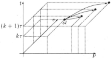
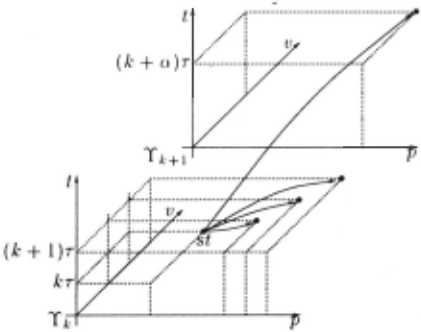
where p is the rad ius of curvature of Y at the current position of A. Constraint (7) is expressed by a velocit.y limit curve in the state space, i.e. the pxv plane. On the other hand , the constraints imposed by the mov­ ing obstacles can be represented by forbidden regions of the pxt space, where t represents the time dimen­ sion [Kant and Zucker, 1986]. In order to deal simu lta­ neously with these two types of constraints, we use the concept. of state-time space [Fraichard, 1993], i.e. the pxvxt space. This concept permits to model simultane­ ously the constraints imposed by the moving obstacles and the constraints on the velocity. Let ST be the state­ time space of A, a curve of ST represents a motion along Y. If such a curve respects ( 6), remains under the ve­ locity limit curve (7) and avoids the forbidden regions due to the moving obstacles, then it is a solution to the Velocity Planning problem. The a lgorithm we designed in order to find such a. curve operates in the following way: it chooses a time-step T and assumes that. the ac­ celeration applied to A during such a time-step is either minimum, null or maximum. Accordingly a. state-time st has three neighbours and a ll the state-times that A can reach from a g iven state-time lie on a regular grid embedded in ST (Fig.:2). This grid is then searched in order to find a sol11t.ion. Accordingly Velocity Planning is reduced to graph search (cf.[Fraicharcl, l\.HJ:3]).

5 Adjacent Paths

This section presents t.he concept. of adjact>nt. paths and shows how it can lw used t.o extend tlw algorithm de­ scribed in the previous section.

5.1 Definition

A path for A is a xy-curve Y of class C 1 whose curvature (wherever it is definNl) is upper-bounded by 1/ f!min. As­ suming that Y does not. intersect itself, a point. P located at a distance from Y smaller than f!m111 has a. unique normal proj ection P' on I. L1, t d 1 ( P) be t.he signed dist.ance 5 between P and its projection 011 I. The path adjacent to Y on its left at a distance f, L is defined as: Y, ={PEW I dy(P) = H} (Fig.:l). Similarly, the path adjacent to Y on its right at a distauee f, /, 1s defined as: Y,. ={PEW I d1(P) = -H}.

Let IN be the nomi11al path leading A to .it.s goal, it is possible to recursively con1put.e a set. of paths adjacent. t.o YN on its left. and on it.s right.. Let. P = {lh~: =

~If Pis on t.heleft (resp. right.) side of Y. t.h('n dy(P) is posit.ive (resp. negative).

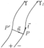
I, ... , n} be the whole set of adjacent paths, Y N in­ cluded. Let us denote by R(Y) the set of points whose distance toY is smaller than f>L/2. The distance f>L be­ tween any two adjacent. paths is chosen so as to ensure that, VYEP:

1. The region swept. by A when it follows a path Y is included in R.(l ).
2. The region swept by A on its left (resp. right) side when it leaves apathY by making a right (resp. left) turn of radius Pmin, is included in R(Y) (Fig.4-a).
3. The region swept. by A on its left (resp . right) side when it reaches a path Y by making a right (resp. left.) turn of radius Pmin is included , in R.(Y) (Fig.4b).

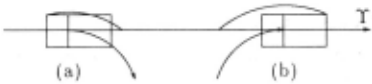
Figure 4: regions swept by A on its left when leav­ ing/reaching a path Y by making a. right turn

As we will see further down , these properties per­ mits to simplify collision checking when A moves along a path (§.5.2) and passes from one path to an adjacent one (§5.3).

5.2 Checking Adjacent Paths

The nominal path is collision-free with the stationary obstacles and respects the kinematic constraints ( 1) and (2) . Unfortunately these two properties do not nec­ essar ily hold for an adjacent path. It may happen that such a path is no longer collision-free or does no longer respect the curvature constraint (2) . Let YEP , it is a mapping [0, v]-· W. Collision and curvature checking lead us to compute a. set of forbidden intervals in the range [0 , ·u] corresponding to parts of Y which violate either of these constraints. Let us denote by p(p) the curvature radius at. position p along Y. The set of for­ bidden intervals for Y is formally defined as:

where Proj ( B;s·. Y) is the projection of the stationary .ob­ stacle B;" on the path Y , i.e. the part of Y which entai ls a collision between A and B; 5 , namely:

where P' is the normal projection of P on 1 and where /1 (resp. /,.) denotes the distance between A's rear axle and it front-most (resp. rear-most) point. Figure 5 depicts an example of forbidden intervals for a path 1 . The interval [a1, bt] corresponds to Proj(Bf ,1) while [a2. b2] corresponds to a part of 1 which does not respect. the curvature constraint. (2) .

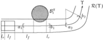
Note that Proj(B/ ,1) is defined by using R(l) in­ st.ead of t.he exac t. region swept. out. by A wht'n it movf's along 1 . This choice is sound beca use the rq~ion swept. out by A is included in R.(i) (property 1 oflj5.1).

5.3 Path-Changing

Let. us study now how A can move from one pat.h t.o an adjacent. one. i.e. make a path-changing. This is depicted in Fig.6-a . At time t 1 , A shifts smoothly fro111 its current. path 1., to an adjacent. path lk+J . A follows a nominal trajectory nand reaches ik+J at. a certain time t 2 . This type of motion is two-dimensional. However it. is possible to take advantage of t.he proprrt.ies of t.lw adjacent. paths in order to reduce it. t.o a one-dimensional motion.

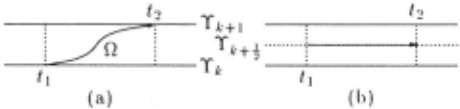
Properties 2 and :3 of 1j5.1 ensure that. , when A mows along n . it. always remains included in t.lw domain R.(Yk )UR.(1k+1 ). Consequf'nt.ly. evaluating whetlwr n is collision-free can lw done very simply hy clwr king out potential collision i 11 both paths I k and I k+ 1 during the time interval [I ·. I:!]. Not.·· that. , in t.his cas··. tlw obst.acles on a pat.h I include both t.he forhidd eu int.er­ vals :F(Y) and t.he projec tions of t.he moving obstacles Proj(BjH (t),Y), such projec tions an' t.inw-dependent..

Accordingly it. is possible t.o model path-changing as a simultaneous motion along lk and lk+J during [IJ , t ::t]. or equivalent.ly, as a three-stage process: (a) at. time t1.

A instantaneously shifts from 11.: t.o a fi ctitious inter­ mediate path ik+l/2· (b) A moves along lJ.:+i/2 dur­ ing [t 1 , t 2] (the obstacles of both lA, and 1k+1 are as­ sumed t.o be projec ted on 1k+1; 2 and (c) at. t.ime t2 , A instantaneously shifts from ik+l/:? to ik+l (Fig.6-b) . Accordingly this modelling reduces path-changing to a one-dimensional motion along a fictitious path .

5.4 Algorithm Extension

The algorithm presented in §4 can easi ly be extended in order to integrate pat.h-changings: a state-time of A simply becomes a 4-t.uple (L, p, v, t) where L is the in­ dex of the current. path of A. Given a method which determines the path-changing trajectory n? it is possible to determine the state-time reached by A at the end of a path-changing. A given state- time has nciw five neigh­ bours: three on t.he same path and two on each adjacent paths . All the state-times reachable from a given state­ time sti ll lie on a regular grid embedded in ST and it is still possible to search t.his grid in order to find a solution (Fig.7).

6 Experimental Results

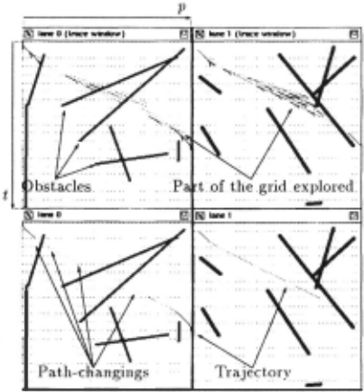
The algorithm presented above has been implemented in C on a Sun SPAHC I. ln these experiments, the mov­ ing obstacles are generated at random without caring whether thev collide with each other . An example with two adjacent paths is depicted in Fig.8. A path is associ­ ated with two windows: a trace window showing the part of t.he grid which has been explored and a result window displaying the final trajectory. Any such window repre­ sent.s t.he ·t.ime x posit.ion ' space of the path . The thick black segments represent. the trails left by the moving ohst.ades and the little clots are points of the underlying grid. Note that. t.he n~ rt. ical spacing of the dots corre­ sponds t.o the t.inw-st.ep r. In the example, A starts on t.he first. path (lane 0) at. position 0 (upper-left corner) with a null velocity. It is to reach the end of the first path (right border) with a null velocity. A can overtake by using the second path (lane 1) .

6 Such a method is described in [Fraichard and Laugier, 19!H) for a car-like robot .

Trajectory -----

Figure 8: an example of trajectory planning with t.wo paths: the solution has four pat.h-changings