
A Stochastic Approach to Qualitative Simulation using Markov Processes
Proceedings of the Thirteenth International Joint Conference on Artificial Intelligence. Qualitative Reasoning and Naive Physics. Pages 1530-1534.
© 1993 International Joint Conferences on Artificial Intelligence
Abstract
Interval based value representation methods constitute a major technical foundation of qualitative reasoning, but they necessarily generate ambiguous situations and spurios solutions. Ambiguity may be reduced by introducing more infonnation and knowlegde: either in the fonn of supplementary quantitative infonnation or by applying general rules, taken from systems theory, on the behavior of dynamic systems. In the second approach concepts as state space diagrams or qualitative cells are exploited. The set of solutions is reduced and general classes of behavior are described. But the concrete behavior still depends on known infonnation, and still too many things cannot be excluded. The application of stochastic concepts could exploit a further type of knowledge: some vague infonnation in the fonn of priorities or the strength of some influence. The concept of Markov processes provides a similar description as the state space approach, but indicates priorities of different behaviors in solution space as well. This paper demonstrates bow existing approaches in qualitative simulation can be transfonned appropriately.
- [Aubin, 1992] Jean-Pierre Aubin. Dynamical Qualitative Simulation. Lecture at Cornett Matari Programme, p. 41, Pavia, Italy, 1992.
- [Berleant and Kuipers, 1990] Daniel Berleant and Benjamin Kuipers. Combined Qualitative and Numerical Simulation with Q3. In Fourth International Workshop on Qualitative Physics, pages 140-152, Lugano, Switzerland, 1990.
- Berleant. 1989]
- Daniel Berleant. A Unification of Numerical and Qualitative Model Simulation. In Workshop on Model Based Reasoning. Proceedings of the Eleventh International Joint Conference on Artificial Intelligence, pages 91-96, Detroit. Mich., 1989.
- [Freedmann, 1971] David Freedmann. Markov chains. Holden Day, San Francisco, 1971.
- [Guariso et al., 1989] Giorgio Guariso, Luigi Nisoli, Andrea Rizzoli, and Hannes Werthner. QUALSIM: An Object-Oriented Software Package for Qualitative Modelling and Simulation. In: G. Iazeolla. A. Lehmann, and H.J Van den Herik (eds.). Simulation Methodologies, Languages and Architectures and AI and Graphics for Simulation. Proceedings of the European Simulation Multiconference, pages 175-180, Rome, Italy, 1989.
- [Guariso et al., 1992] Giorgio Guariso, Andrea Rizzoli, and Hannes Werthner. Identification of Model Structure via Qualitative Simulation. IEEE Trans. on SMC 22 (5): 1075-1086, 1992.
- Ishida. 1989] Yoshiteru Ishida. Using Global Properties for Qualitative Reasoning: A Qualitative System Theory. In Proceedings of the Eleventh International Joint Conference on Artificial Intelligence, pages 1174- 1179, Detroit. Mich., 1989. IJCAI
- Ishida. 1992]
- Yoshiteru Ishida. A Graphical Approach to Qualitative Reasoning on Dynamic Systems. In Proceedings of the Tenth European Conference on Artificial Intelligence, pages 744-748, Vienna, Austria. 1992.
- [Kuipers, 1985] Benjamin Kuipers. The limits of Qualitative Simulation. In Proceedings of the Ninth International Joint Conference on Artificial Intelligence, pages 128-136, Los Angeles, Cal., 1985. IJCAI
- [Kuipers, 1986] Benjamin Kuipers. Qualitative Simulation. Artificial Intelligence 29: 289-388, 1989.
- Kuipers and Berleant. 1988] Benjamin Kuipers and Daniel Berleant. Using Incomplete Quantitative Knowledge in Qualitative Reasoning. In Proceedings of the AAAI-88, pages 324-329, Saint Paul, Minn., 1988.
- [Kuipers and Chiu, 1987] Benjamin Kuipers and Charles Chiu. Taming Intractible Branching in Qualitative Simulation. In Proceedings of the Tenth International Joint Conference on Artificial Intelligence, pages 1079- 1085, Milan, Italy, 1987. IJCAI
- [Kuipers et al., 1991] Benjamin Kuipers, Charles Chiu, David Daile Molle, and D.R. Throop. Higher-order derivative constraints in qualitative simulation. Artificial Intelligence 51: 343-379, 1991.
- [Lee and Kuipers, 1988] Wood Lee and Benjamin Kuipers. Non-Intersection of Trajectories in Qualitative Phase Space: A Global Constraint for Qualitative Simulation. In Proceedings of the AAAI-88, pages 286-290, Saint Paul, Minn., 1988.
- [Pearl, 1986] Judea Pearl. Fusion, Propagation and Structuring in Belief Networks. Artificial Intelligence 29: 241-288, 1986.
- [Peot and Shachter, 1991] Mark A. Peot and Ross D. Shachter. Fusion and propagation with multiple observations in belief networks. Artificial Intelligence 48: 299-218, 1991.
- [Pflug, 1986] Georg Pflug. Stochastische Modelle in der Informatik (in German). B.G. Teubner, Stuttgart. 1986.
- [Sacks, 1990a] Elisha Sacks. Dynamic Systems Perspective on Qualitative Reasoning. Artificial Intelligence 42: 349-362, 1990.
- [Sacks, 1990b] Elisha Sacks. Automatic Qualitative Analysis of Ordinary Differential Equations Using Piecewise Linear Approximations. Artficial Intelligence. 41: 313-364, 1990.
- [Scheines et al., 1991] Richard Scheines, Peter Spirtes, and Clark Glymoure. A Qualitative Approach to Causal Modeling. In: Paul A. Fishwick and Paul A. Luker (eds.) Qualitative Simulation, Modeling and Analysis. Advance in Simulation 5, pages 72-97, Springer, New York, 1990.
- [Shen and Leitch, 1990] Quiang Shen and Roy Leitch. Integrating Commonsense and qualitative simulation by the use of fuzzy sets. In Fourth International Workshop on Qualitative Physics, pages 221-232, Lugano, Switzerland, 1990.
- [Shen and Leitch, 1991] Quiang Shen and Roy Leitch. Extending the Quantity Space in Qualitative Reasoning. In First European Workshop on Qualitative Reasoning about Physical Systems, pages 13, Genova. Italy, 1991.
- [Struss, 1987] Peter Struss. Problems of Interval Based Qualitative Reasoning. Technical Report Siemens #INF2ARM-87, 18, 1987.
- [Struss, 1988] Peter Struss. Global Filters for Qualitative Behaviors. In Proceedings of the AAAI-88, pages 275- 279, Saint Paul, Minn., 1988.
- [Wellman, 1988] Michael P. Wellman. Qualitative Probabilistic Networks for Planning under Uncertainty. In: John F. Lemmer and Laveen N. Kanal L.N. (eds.) Uncertainty in Artificial Intelligence 2. Machine Intelligence and Pattern Recognition 5, pages 197-208, North-Holland, Amsterdam, 1988.
- [Yager et al., 1987] R.R. Yager, S. Ovchinnikov, R.M. Tong, and H.T. Nguyen. Fuzzy Sets and Applications: Selected Papers by LA. Zadeh. Wiley, New York, 1987.
References were extracted automatically from the PDF and may contain errors.
Full text extracted automatically from the PDF; figures, tables and equations may differ. The PDF is the version of record.
1 Introduction
Interval based value representation methods constitute a major technical foundation of qualitative reasoning, but they necessarily generate ambiguous situations and spurios solutions [Struss, 1987; Kuipers, 1985; Kuipers, 1986]. Ambiguity may be reduced by introducing more infonnation and knowlegde: either in the fonn of supplementary quantitative infonnation [Kuipers and Chiu, 1987; Kuipers and Berleant, 1988; Berleant, 1989; Berleant and Kuipers, 1990] or by applying general rules on the behavior of dynamic systems [Lee and Kuipers, 1988; Kuipers et al., 1991; Struss, 1988]. Since qualitative reasoning deals with dynamic systems, similar to systems theory, concepts of the latter field can be applied. The works of [Sacks, 1990a; Sacks, 1990b; Ishida, 1989; Ishida, 1992; Aubin, 1992] which exploit state space diagrams, the course of trajectories or the concept of qualitative cells justify this correspondence. These approaches describe the side the result of the reasoning process may denote priorities on the different possible behaviors as well.
QUALSIM, based on fuzzy sets, may serve as an example to demonstrate the feasibility of the proposed approach. QUALSIM [Guariso et al. , 1989; Guariso et al., 1992] is based on influence diagrams. Causality is identified in the modelling process and compiled into the model. The algorithm can be seen as a constructive one, dedicated to the straightforward generation of a qualitative behavior of a system. In close relationship to numerical simulation time is considered as an integer counter, a unit increment corresponding to a computation step. This may or may not indicate a change of the system's state.
The value of a state variable may take one of the following labels from the set Q of qualitative values:
- +1- EXTRALARGE
- +1- LARGE
- +1- MEDIUM
- +1- SMALL
- +1- EXTRASMALL
ZERO
QUALSIM assumes that the entire range of possible values of a variable can be defined in advance. This representation covers the whole range, it is finite, ordered and associative excluding the extreme intervals on both sides. But this is no hard restriction since the knowledge of the entire range is assumed to exist. Thus, each variable x is identified by a numeric range Rx defined as a subrange of the real number space. Each value of the magnitude is a fuzzy set defined by delimiting values vk, k= 1, ... ,12 (by default the vk's are evenly spaced in the positive and negative subintervals of R) and a tuple (vk· a, b) defining a fuzzy membership function J.1A (x) (similar to [Shen and Leitch, 1990; Shen and Leitch, 1991] and different to the original notion of QUALSIM):
for each k and the corresponding A e Q. In the case of the two delimiting points v 1 and v 12 J.1A(x) remains at a value of 1.
The constant d is defined global and determines, together with the variable dependent values a and b, the fuzzyness of the qualitative values.
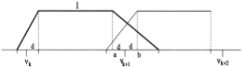
Connections between two variables may possess one of the following labels:
- +1- EXTRASTRONG
+1- STRONG
+1- MEDIUM
+1- WEAK
+1- EXTRAWEAK
These labels are assumed to correspond to numeric subranges of the interval [ -1, 1]. They are instantiated to specific numeric values c 0 ij randomly distributed in the respective subrange. The probability distribution of these values is normal and centered on the center of the subrange. Standard deviation crij is chosen by the user in order to reflect his/her subjective perception of the uncertainty of the connection. For instance, if the user selects the default value crij=O, the distribution is reduced to an impulse and represents a high confidence in the appropriateness of the selected value. For simplicity, in the following we will only consider this case. Thus a kind of an influence graph is constructed [Scheines et al .· 1991] (see figure 2), indicating the strength of a connection and not its probability (as in [Wellman, 1988; Pearl, 1986; Peot and Shachter, 1991]).
The algorithm is based fundamentally on the conversion of qualitative values into quantitative ones and vice versa. The propagation of the uncertainty during the simulation is represented by the bifurcation of the simulation tree.
- At the beginning of the simulation the initial qualitative value for state variable x is transformed into its numeric equivalent x 0 being the characteristic point of the relative fuzzy set (i.e. its center).
- Given a qualitative value xi(t) and numeric value x 0 i(t) for the state variable at time t and assuming that Ii = { xj : xj is connected to xi· j e 1.. n} is the set of variables that exert an influence on the variable xi, the new numeric value is computed as
and c 0 ij is the mean value of the connection between xi and xj and Rx is the range of the respective variable.
- Since QUALSIM distinguishes between state and output variables, the latter ones are calculated similarity to state variables. It follows that the influencing arcs of QUALSIM represent either an integration step (when state variables are influenced) or in the case of output variables just an influence. Given a qualitative value Yi(t) and its numeric value y 0 i(t) for the output variable at time t, assuming again that Ki = {xj : xj is connected to Yi· j e 1.. n} is the set of variables that exert an influence on Yi· the new numeric value is computed as
Y? (t+l)= L t:.xp) and ll.xj is calculated as before. jeKI
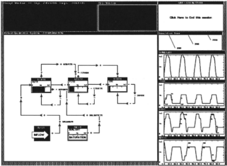
- The numeric value of a variable is transformed again into a qualitative value:
- If the membership grade of x 0 (t+1) exceeds a predefined threshold l!'(x) at least in one of the sets (i.e. if x 0 (t+ 1) belongs to the 1-1'-cut of at least one of the sets), the new qualitative value assigned to xi is the label of the set where x 0 (t+ 1) bas the highest membership grade.
- If all the membership grades are lower than 1-1', an ambiguity occurs and either the user is asked to assign the qualitative value by choosing between the one at time t and the higher (lower) value depending on the sign of l:j ~xj or a fixed strategy like depth or breadth first is applied.
- If the qualitative value of a state variable computed with the above procedure is different from the one at time t, the corresponding numeric value x 0 (t+ 1) is equal to the characteristic value of the relative set. Otherwise, the qualitative derivative (i.e. the sign of the term l:j ~xj) is taken into account and the term
is added to x 0 i(t+ 1). p is the number of time steps with variable xi(t) in the same qualitative state with positive increments, and m is the number of time steps with negative increments. When a state variable enters a new qualitative state it inherits the last value of the qualitative derivative.
These steps are repeated till the time counter reaches a predefined value. An important feature is, that to avoid calculating the entire simulation tree the user may define in an ambiguous situation with which branch to proceed (this may also be defined automatically as depth or breadth first, or randomly).
This constructive approach to qualitative reasoning can now be mapped without loss of information to the formalism of QSIM 1 [Kuipers, 1986] and it is also possible to derive an interpretation based on Markov chains. The latter one will be elaborated in the following.
3 Markov Processes
Given the set of random difference equations of QUALSIM a matrix of transition probabilities between states can be generated. Such a matrix describes, similar to approaches in systems theory, the state space of a system, independent of distinct initial values. But in difference to the state space description where each of the described . behaviors is possible (the distinct trajectory depends on initial and parameter values), a description in form of Markov cbains 2 defines priorities between transitions as well, though the concrete behavior still depends on known initial and parameter values.
The Markov property of a system says that the state of a system depends just on its predecessor state. X 1 , .. , X 0
1 This is shown by a working paper of the authors, not yet ~ublished .
In this paper we use the concept of finite, in contrast to infinite, Markov chains. Moreover, we do not discuss the case of possibilistic automata, which can also be described by the means of Markov processes.
being random variables and S the finite set of states then a Markov chain is a sequence of the random numbers where P[X 0 = sj I X 1 , ... ,X 0 _.J = P[X 0 = sj I X 0 _.J. Homogeneous Markov chains do not depend on n, i.e. p .. = P[X = S· I IJ n J ~n-I = si] does not depend on n (pij is independent from ume; see [Freedman, 1971; Pflug, 1986]). This is the probability that the system changes from state si to state s .. These probabilities can be written in the form of ~ quadratic matrix P indicating the state transition probabilities for all combinations of states. The rows of this matrix sum up to 1, i.e. a state has to change to its successors. The initial situation can be described by a row vector v, i.e. v is a probability distribution describing the probability of each state being initial state. Multiplying v with P gives a vector w, i.e. w = v"' P, which describes the probability of the system being in a specific state after the first transition, at the second time point. In a stationary case v = w, the probabilities are not changed by applying P. Matrix P describes the transition probabilities in one step, multiplying P with P, the transition table is generated for two steps. Thus, pn describes the transition probabilities of applying n transitions, i.e. the situation of the system after n steps.
Matrix P has some nice properties, for example it classifies the states into equivalence classes. A state S· may be reached from si if 3 nand n > 0, that Pr 0 > 0 (writlen as si ~ sj; this is no logical implication!), otherwise it cannot be reached from S 1 ·· If both s- ~ s- and s- ~ s- are valid I J J I ' then si and sj are called equivalent (si ~ s-). Those states which are equivalent to each other form ~ equivalence class. If the system has left an equivalence class once, it can never return. Such classes are partially ordered by the following definition: G 1 is before G 2 if 3 si e G 1 and 3 sj e G 2 and si ~ sj . Thus, not only probabilities for specific behaviors may be derived from a transition matrix, but the sequence of visited states or the existence of cycles can be indicated as well.
4 Markov Processes in Qualitative Simulation
The application of this method to the QUALSIM approach requires the consideration of some problems:
- the fuzzy number representation of QUALSIM has to be converted to a probabilistic form to guarantee some Markov properties,
- QUALSIM denotes the strength of an influence between variables, no state description is given in advance,
- the entire set of possible system states is not known.
The solution of the first point makes a "normalized" representation of the qualitative values necessary, i.e. LAJ.lAeQ(x) = 1 for every x e Rx, i.e. fuzzy numbers are transformed in order to represent probabilities.
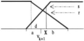
Such a transformation has to maintain the reletaionship between the two fuzzy numbers, i.e. if x is the current value of the respective state variable the following has to be satisfied:
The important feature is the relationship between both values and not their magnitudes.
The second and the third problem can be discussed together: The set of system's state S can be constructed in advance based on the limited value set of the qualitative quantity space. If w = #(W) denotes the number of state variables (W is the set of state variables) and u = #(Q) the number of qualitative values, then the number of all possible states is uw. Therefore, the setS can be generated by enumerating all possible value combinations for each element of W. Each element of S is a vector, the first member of the vector representing the value of the first variable, the second member representing the value for the second state variable, and so on. Every value combination represents a state and for every combination of values the respective state can be identified. Thus, the finite state space is constructed.
succ(m I m e Q) denotes the neighbour which follows a member of Q, and pred(m I m e Q) the neighbour which preceeds a member of Q. LARGE is succ(MEDIUM) and SMALL is pred(MEDIUM). succ(EXTRALARGE) is defined to be EXTRALARGE, pred( -EXTRALARGE) is - EXTRALARGE again. The transition probabilities Ps·s·· i.e. going from state si to state sj can now be derived <§tk denotes the kth COmponent Of vector Si - With Sik E Q - and G denotes the distribution of the numerical correspondents ~k of a qualitative value sik): 3
The probability to change from Si to S- - the system is in Si at time t and in Sj at time t+ 1 - is z~ro when the law of continuity is violated. Riq correspond to those components q (i.e. state variables) that influence the state variable k of W. The second part represents the original formula to calculate the new value of a state variable where the quantitative correspondent of a qualitative value is weighted by the respective probability distribution. Based on the fact that variables vary continuously, it follows that P is very sparse. Every state Si may just have 3w successors since in each transition just three possibilities of change for each state variable exist, i.e. in each row of P a small number of elements is *- 0.
3 G can be obtained by applying the model equations to produce the trajectory of the system. Depending on the cr this trajectory takes only a finite number of quantitative val3es inside each qualitative range. Each of these points has thus a well defined probability of occurrence.
Since Ps·S·k represents just the kth component of a vector of probabhlties several approaches can be applied to approximate the overall probability to go from si to sj.
a) Since the decisions of choosing a specific range for each component of a state variable are independent, in cases where the state variables are only loosely coupled the multiplication of the single components of the probability vector is a reasonable operation, i.e. Psis· = nk Pijk· Rewriting Ps·s· as Pw the Markov property of:Ej e succ(Si) Pij = I can be d~d10nstrated as described in the following.
The single Pijk elements can be grouped as a matrix with dimension w x 3w, w is the number of state variables:
| S1 | Sz | S3 | S3w |
|---|---|---|---|
| Pill | Pi2l | Pi3l | Pi3Wl |
| Si Pil2 | |||
| Pilw | Pi2w | Pi3Ww |
If w = 1 then Si has just 3 successors Sj which depend on the value of St either pred(Si) or Si or succ(Si). Given the initial normaltsation of the membership functions these three probabilities sum up to 1.
Now, assuming that the above formula is true for the number of state variables being n, it can be shown that it holds for the number being n+ I as well. The respective matrix is obtained by adding one row for the probabilities of state variable n+ 1 which triples the number of columns:
| Pir!D+l | Pir!D+l | Pir2D+l | Pir2n+l | PirJD+l | Pir3n+l |
| Pill | Pi3Dl | Pill | Pi3°l | Pill | Pi3°l |
| Pil2 | Pil2 | Pil2 | |||
| Piln | Pi3°n | Piln | Pi3°n | Piln | Pi3°n |
Pir 1 n+ 1 is the probability that variable n+ 1 does not change its value at the next state, Pir 2 n+ 1 that the next value is succ(Sin+1), pir3n+l that the next value is pred(Sin+l). The sum of these three sum up to 1. By
1 = Pi1jn+1 X 1 + P;rln+l X 1 + P;rln+) X 1 =
and by modifying the indices, for example Pirin+l = Pijn+l' and by changing the order of summation and multiplication
w = n+ 1. Thus the Markov property is satisfied.
b) Instead of multiplying the components of the probability vector, the minimum of the components could be chosen. This would mean that the most unlikely case inside each column determines the overall probability of this specific transition. The inertest variable determines the behavior of the system. In this case a strong dependence between the state variables is assumed. To obtain the Markov property every single value has to be weighted by the row sum of all minima, i.e.
c) As a final approach the single components of each vector could be added. Also in this case we assume a strong dependence between the model's variables. A possible interpretation would be some kind of averaging the transition probabilities which of course makes only sense if no component has a probability of zero. In this approach the value can be calculated by the following formula Pij = 1/F w * :Ek Pijk·
The factor F w represents the sum over all components of Pij for all successor states Sj of Si, i.e. :Ek :Ej esucc(Si) Pijk = Fw, where Fw is defined recursively: F0=0 and Fi=3*Fi-l + 3i-l, \;/ i > 0. This can be easily proved by induction similar to the case of multiplication. Now the row sum of P is 1, satisfying the Markov pro}lerty of :Ej Pij = 1.
5 Conclusions
The choice of the method to compute the single probability still has to be explored. It can be assumed that the concept of reachability and velocity of reaching specific states will depend on this choice. And it has to be confronted with the simulation results of the original approach.
The matrix P represents the state space of the system and the simulation of a system is now done by multiplications of matrices and vectors, describing the initial state of the system. These are simple operations, but the dimension of the matrix - even if it is very sparse - may be enormous. However, it can be built in advance and provides a description of the state space indicating privileged behaviors. Moreover, it can be used to divide the state space into equivalence classes, giving a qualitative interpretation of the whole state space. This work shows that, given uncertain information in the form of possibilities or probabilities, this information can be used by the means of Markov processes to generate the entire set of solutions, denoting priorities among them as well.
@inproceedings{ijcai1993p212,
  title     = {A Stochastic Approach to Qualitative Simulation using Markov Processes},
  author    = {Grossmann, Wilfried and Werthner, Hannes},
  booktitle = {Proceedings of the Thirteenth International Joint Conference on
               Artificial Intelligence, {IJCAI-93}},
  publisher = {International Joint Conferences on Artificial Intelligence},
  editor    = {Ruzena Bajcsy},
  pages     = {1530--1534},
  year      = {1993},
  note      = {Qualitative Reasoning and Naive Physics},
  url       = {https://ijcai.org/proceedings/1993/212},
}
TY - CPAPER TI - A Stochastic Approach to Qualitative Simulation using Markov Processes AU - Grossmann, Wilfried AU - Werthner, Hannes T2 - Proceedings of the Thirteenth International Joint Conference on Artificial Intelligence, IJCAI-93 PB - International Joint Conferences on Artificial Intelligence PY - 1993 SP - 1530 EP - 1534 UR - https://ijcai.org/proceedings/1993/212 ER -Copied
Machine-readable versions of this paper, for tools and AI agents:





