
The Limits of Qualitative Simulation
Proceedings of the Ninth International Joint Conference on Artificial Intelligence. Automated Reasoning. Pages 128-135.
© 1985 International Joint Conferences on Artificial Intelligence
Abstract
Qualitative simulation is a key inf<>r<'nce proc!'s~ in qualitative ramal rmsoning. In this pap!•r, W<' pr!'sent th!' QSIM algorithm, a new algorithm for qualitative simulation that grneralir.Ps the best features of existing algorithms, and allows direct comparison~ among alternate approaches. QSIM is an efficient constraint-satisfaction algorithm that can follow either its standan! semantics allowing the creation of new landmarks, or the { +, 0 ,- } semantics where 0 is the only landmark value, by changing a table of legal state-transitions. We argue that the QSIM semantics make more appropriate qualitative distinctions since the {+, 0, -} semantics can collapse the distinction among increasing, stable, or decreasing oscillation. We also show that (a) qualitative simulation algorithms can be proved to produce every actual behavior of the mechanism being modeled, but (b) existing qualitative simulation algorithms, because of their local points of view, can predict spurious behaviors not produced by any mechanism satisfying the structural description. These observations suggest specific types of care that must be taken in designing applications of qualitative causal reasoning systems, and in constructing and validating a knowledge base of mechanism descriptions.
- J . de Kleer. 1977. Multiple representations of knowledge in a mechanics problem-solver. Proceedings of the Fifth Inter- national Joint Conference on Artificial Intelligence. IJCAI
- J. de Kleer. 1978. Causal and teleological reasoning in cir- cuit recognition. MIT Artificial Intelligence Laboratory TR- 529.
- J. de Kleer. 1979. The origin and resolution of ambiguities in causal arguments. Proceedings of the Sixth International Joint Conference on Artificial Intelligence. Tokyo, Japan. IJCAI
- J . de Kleer and D. G. Bobrow. 1984. Qualitative reasoning with higher-order derivatives. In Proceedings of the National Conference on Artificial Intelligence ( AAAI-84}. Los Altos, CA: William Kaufman.
- J. de Kleer and J . S. Brown. 1983. The ongm, form, and logic of qualitative physical laws. In Proceedings of the Eighth International Joint Conference on Artificial Intelli- gence . Los Altos, CA: William Kaufman.
- J. de Kleer and J . S. Brown. 1984. A qualitative physics based on confluences: Artificial Intelligence 24: 7 -83.
- K. D. Forbus. 1981. Qualitative reasoning about physi• cal processes. In Proceedings of the Seventh International Joint Conference on Artificial Intelligence . Los Altos, CA: William Kaufman.
- K. D. Forbus. 1983. Measurement interpretation in quali- tative process theory. In Proceedings of the Eighth Interna- tional Joint Conference on Artificial Intelligence. Los Altos, CA: William Kaufman. IJCAI
- K. D. Forbus. 1984. Qualitative process theory. Artificial Intelligence 24: 85 -168.
- K. D. Forbus. 1984. Qualitative process theory. Ph.D. the- sis, MIT Department of Electrical Engineering and Com- puter Science.
- D. Gentner and A. Stevens, (Eds.). 1983. Mental Models. Hillsdale, NJ: Erlbaum.
- P .• J. Hayes. 1979. The naive physics manifesto. In D. Michie (Ed.), Expert Systems in the Micro-electronic Age. Edinburgh: Edinburgh University Press, 1979.
- B. J. Kuipers. 1982. Getting the envisionment right. In Proceedings of the National Conference on Artificial Intelli- gence {AAAI-82}. Pittsburgh, Pennsylvania, August 1982.
- B. J. Kuipers. 1984. Commonsense reasoning about causal- ity: deriving behavior from structure. Artificial Intelligence 24: 169 -204.
- B. J . Kuipl'rs. 1985 . . Qualitative Simulation of Mecha- nisms. Cambridge, MA: MIT Laboratory for Computer Sci- ence TM-274.
- B. J. Kuipers and .T. P. Kassirer. 1983. How to discover a knowledge represPntat.iou for causal reasoning by studying an expert physician. In Proceedings of the Eighth Interna- tional Joint Conference on Artificial Intelligence. Palo Alto: William Kaufman.
- B. J . Kuipers and J . P. Kassirer. 1984. Causal reasoning in medicine: analysis of a protocol. Cognitive Science 8: 363-385.
- B. Williams. 1984a. The usc of continuity in a qualita- tive physics. In Proceedings of the National Conference on Artificial Intelligence (AAAI-84}. Los Altos, CA: William Kaufman.
- B. Williams. 1984b. Qualitative analysis of MOS circuits. Artificial Intelligence 24: 281 -346.
References were extracted automatically from the PDF and may contain errors.
Full text extracted automatically from the PDF; figures, tables and equations may differ. The PDF is the version of record.
1 Introduction
An <'Xp(·rt system is often a "shallow modd" of its application domain, in the s<>nsc that conclusions arc drawn directly from ob servable fpatures of the prl's('llted situation. Many researchers be lieve that genuinely expert performance must also rest on know l edge of "def'p models," in which an underlying mechanism, whose state variables may be not. be directly observable, accounts for the observable facts [11] .
One major line of research toward the fl)presentation of deep models is the study of qualitative causal models [1-19]. Research on qualitative causal models differs from more general work on deep models in focusing on qualitative descriptions of the deep mechanism, capable of representing incomplete knowledge of the structure and behavior of the mechanism. Symbolic manipula tion of qualitative descriptions alsn corresponds well with expla nations by human experts [16,17].
1 This research was supported in part by the National Library of Medicine through NIH Grants LM 03003, LM 04125, and ROI LM 04374, and by the National Science Foundation through grants MCS-8303640 and DCR8417934.
THE LIMITS OF QUALITATIVE SIMULATION
Benjamin Kuipers
MIT Laboratory for Computer Science, Cambridge, Massachusetts 02139.
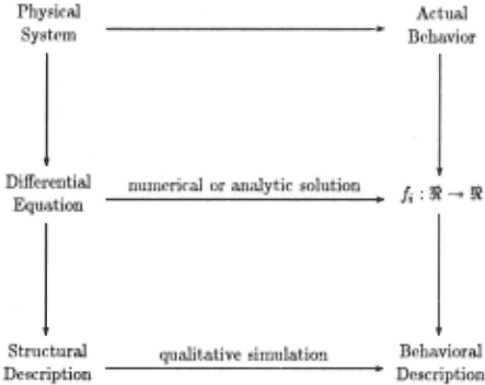
A central inference within this approach is qualitative simu lation: derivation of a description of the behavior of a mechanism from a qualitative description of its structure. Differential equa tion~ provide a useful comparisou. A differential equation de scribes a physical system in terms of a set of state variables and constraints. The solution to the equation may be a function rep resenting the behavior of the system over time. The qualitative structural description is a further abstraction of the same system, and qualitative simulation is intended to yield a corresponding abstraction of its behavior (figure 1).
All qualitative simulation systems predict multiple possible behaviors given certain structural descriptions and iuitial condi tions. Researchers in this area (myself included) have hoped to prove that the predicted behaviors iuclude all and only the possi ble behaviors of r"al mechanisms satisfying the given description. Half of this is correct: we cau prove [15] that qualitative simula t.ion cannot miss any actual behavior. Howcvl'r, because of the local nat. uri' of it.s dedsion criteria, qualit.at.ive simulation can pre dict hd1aviors that. arc not. possiblP for any rmluH·chanism satis fying the given dPscript.ion, and we construct. a counterexample. We discuss the implications of these results for the construction of a qualitative causal reasoning system.
The QSIM algorithm has bel'n implemented in Lisp on the Symbolics 3600, and all examples in this paper have been run, as well as numerous others in elementary physics, nephrology, and cardiology.
1.1 Overview
This S<'rtion provid<·s au ov<'rvicw of qualitative simulation and the QSIM algorithm. Some of t.hes<' roucepts are defined more formally below. The cmupl!'t.e formal trcat.uwnt is pre sented in [15]. Qualitative simulation of a system starts with a description of the known st.ruct.nrc of th<' system and its initial state, and produc<'s a tree consisting of the possible future states of the system. Tlw possible behaviors of the system are the paths from the root of this tree to its leaves.
The structural description consists of a set of symbols r<'presenting the physical parameters of the system (contin uously differentiable real-valued functions of time), and a set of constraints on how those paramet.ers may he related to each other. The constraints are two- or three-place relations on phys ical parameters. Some specify familiar mathematical relation ships: DERIV(vel, ace) , ADD(nct, out , in) , MU LT(ma88, ace, force), MIN U 8 (! wd, rev). Others assert qualitatively that there is a functional relationship between two physical parameters, but only specify that. the relationship is monotonically increas ing or decreasing: M +(price , power) and M " (mph,mpg) . The constraints are design<'d to permit a large class of differential equations to be mapped straight-forwardly into structural de scriptions.
Each physical parameter is a continuously differentiable real valued function of time with only finitely many critical points. Its value at any given point in time is specified qualitatively, in terms of its relationship with a totally ordered set of landmark values. Every critical value of the function is a landmark value. The landmark values may be described either numerically (e.g. zero) or symbolically; t.heir ordinal relationships arc their essen tial properties. As the quali tative simulation proceeds, it can discover new critical points and thus add new landmark values to the sequence. The qualitative state of a parameter consists of its ordinal relations with the landmark values and its direction of change.
Tinl!', within om' po~sihl<' h<'havior, is represented as a to tally or<l<'r!'d set of ~ymbolir distinguished time-points. The cnrn·nt time i~ t·it.hcr at or bct.w('en distinguished time-points. All of the time-points are generated as a result of t.IH' qualitative simulation process.
At a distinguished time-point. if several physical parameters linked by a sing!<' constraint an· equal t.o landmark values, they are said to havP corresponding values which can be repre sented and used by tlH' qualitative simulation. Corresponding values providl' additional qualitative constraints on the behav ior of structural relationships otherwisc described only as M + or M -. The rase of corr<'sponding values (0, 0) is sufficiently com mon to justify the special notation, !vfrj and M 0 - . When zero is the only landmark, useful corresponding values are seldom dis covered.
A set of constraints on the physical parameters of the system is only valid in some operating region, defined by the legal ranges of values that some parameters may take on. The le gal range of a parameter is a dosed interval whose endpoints are landmark values of that parameter. These endpoints may be associated wi th transitions to other operating regions where a different set of ·constraints apply. The operating regions are designed as an interface to Forbus' [8,10] concept of processes, but that topic is beyond the scope of this paper.
TIH' initial state of tlw system is d!'fiiH'd J,y til!' opPrating rq;ion and a s<'l of qualitativ!' vahu·s for tlw phy,iral param <·ter:<. Th<' qualitative simulation j>ron·c·ds by <l<'l<'rmining all of th<' po:<sihk rhangC's in qualitative va]uC' permitted to each paramcl.<'r. then Iii tniug the combinatiom hy applying progres sively hroad<'r rouM.raints. lf more than one qualitative change is possible, the current state has multiple successors, and the simulation produces a tree.
Two qualitative states in the same operating region are iden tical if all paranwters arc equal to the same landmark values, and all thf' directions of change an· the same. If a state is identical to a direct. predecessor, a cyclic behavior can be recognized.
2 Qualitative Behavior
In t.hi~ section, we present a more rigorous definition of quali tative description of continuous hehavior, leading up to the QSIM algorithm and several theorems characterizing its strengths and limitations.
We reluctantly contribute to the proliferation of notations for qual it ativc description of continuous fuuctions. The advantages of th<' uotation used here arc that. it. ( 1) naturally allows for an arbitrary and changing set of laudmark values, (2) uses a single term for the qualitative description of a function's maguitude and derivative, and (3) emphasizes that the qnalitativc description of the derivative is of low and fixed n·solut.ion, while qualitative description of magnitude is of higher and possibly changing res olution.
Definition 1 . Let f : [a, b] -+ !R' be a continuously differ entiable function with only finitely rrumy critical points in [a, b]. The landmark values off are a finite set l1 < · · · < lk of values in the range of f including all its criti~al value.s. The landmark values alw1tys include { -oo, 0, oo}. The distinguished time points of f are a finite set of t; E [a, b] including all points where f takes on a landmark value.
Definition 2 . Let !1 < · · · < lk be the landmark VILlue.s of f : [a, b] -· ~JI'. For any t E [a, b], (JS(J. t). the qualitative state off at t , i.s a 1mir {qval , qdir) , dcji11ed as follows:
Definition 3 . For adiacent distingui.shed time-points t; and ti+l, dcfinr. QS(f. t; , ti+l ), the qualitative state off on (t;, t;+J), to be QS(J, t) for any t E (t;, I;+ I).
The Intermediate Value and Mean Value Theorems allow us to show that this definition is well-founded.
Definition 4 The qualitative behavior of f on lc1, b] is the sequence of qualitative states off:
an alternating sequence of qualitative .1tates at distinguished time points, and on intervals between distinguished time-points.
Definition 5 A system is a set F = {h ... /m} of/unctions/; : Ia, b] -> lR*, each with it., own set of landmarks and distinguished time-point.,. The distinguished time-points of a system F are the union of the distinguished time-points of the individual functions /; E F. The qualitative state of a system F of m functions is the m-tuple of individual qualitative states:
The qualitative behavior of F is the sequence of qualitative states ofF:
If t; and/or ti+l are not distinguished time-points of a par ticular /j , then t; and the interval (t; , t;+J) must be between two distinguished time-points of /j , say tk and tk+l· Then QS(fi>t;) ami QS(fj, t;, t;+!) are defined to be the same as the containing. QS(fi, tk, tk+t)·
A coutiuuously differeutiable function f : Ia, b] -> !R* is restricted to tlw following set of possible transitions from one qualitative state to the next.
P-Transitions
| Name | QS(!, t;) | => | QS(!, t;, ti+t) |
| P1 | (lj,std) | (lj, std) | |
| P2 | (lj, std) | ((lj, lj+J), inc) | |
| P3 | (lj, std) | ((lj- 1, lj), dec) | |
| P4 | (lj, inc) | ((lj, lj+J) , inc) | |
| P5 | ((lj,lj+l),inc) | ((lj, lj+J), inc) | |
| P6 | (lj,dec) | Wi - 1• 13 ), dec) | |
| P7 | ((lj, lj f t), dec) | ((lj, lj+J), dec) |
1-Transitions
| 11 | (lj, std) | (lj, std) |
| 12 | ((lj, lj+I), inc) | (li+l> std) |
| 13 | ((li,l 3 +!), inc) | (lj+l> inc) |
| 14 | ((1j,1 3 +J), inc) | ((/j,lj+!),inc) |
| 15 | ((lj, li+l), dec) | (lj,std) |
| 16 | ((lj,lj+l),dec) | (lj, dec) |
| 17 | ((lj , li+l), dec) | ((lj, Lj+J), dec) |
| IS | ((lj, lj+J), inc) | (1', std) |
| 19 | ((lj, Lj+J), dec) | (I*, std) |
In cases JS and 19, f becomes std at I*, a new landmark value such that lj < I* < lj+l· In these cases, a previously unknown landmark value is discovered because other coustraints force f'(t) to become zero.
Th!'se <lefinitious giv<' 11s a precis<· st·mautics for t.}l(' qllalita tiv<' <ksniptiou of coutiuncms f11nrtious. ami rlarifi<·s the concept of the ··next state." Ev<'ry stat.!' has a <jllillit ative d!'srription QS(F, t), but that clescriptimJ rhang<·s ouly at discret!' distin gHish!'d time-points, and rcmaius constaut 011 the open intervals b!'t.w<'cn them. Thus the "next state" of a mechanism is more properly called the next di.1tinct qualitative state description of the mechanism.
2.1 Qualitative State Transitions
The Intermediate Value Tlworem and the Mean Value The orem restrict the way a continuously differentiable function can change from one qualitative state to the next. There are two types of qualitative state transitions: P-transitions, moving from a time-point to a time-interval, and !-transitions, moving from an interval to a point. Table 1 specifics the set of possi ble transitions that can take place in the qualitative behavior of a single function. The table takes into account the possibility that not all landmark values are currently known, so that a new critical point might be discovered (IS and 19).
3 Qualitative Simulation
The qualitative simulation al~orithm determines the possible qualitative behavior descriptions consistent with the initial state and the structural constraints. It is given the following structural description of a mechanism.
- A set {/1 . .. fm} of symbols representing the physical pa rameters in the system.
- A set of constraints applied to the parameter symbols: ADD(f, g, h) , MULT(f,g , h), MINUS'(!, g) , DERIV(J,g), M+(J,g), and M - (!, y). Each constraint may have associ ated corresponding values for its parameters.
- Each parameter is associated with a totally ordered set of symbols representing landmark values. Each parameter may have upper and lower range limits, which are land mark values beyond which the current set of constraints no longer apply. A range limit may be associated with a new operating region which has its own constraints and range limits.
- An initial time-point symbol, to, and qualitative values for each of the /; at to.
The result of the qualitative sim11lation is one or more quali tative behavior descriptions for the given paramct.ers. Each qual itative behavior description consists of the following:
- A sequence { t0 . .. tn} of symbols representing the distin guished time-points of the system's behavior.
- For each parameter /;. a totally ordered set of landmark values, possibly extending the originally given set.
- For mch parameter, at each distinguished time-point or interval between adjacent tim<'-points, a qualitative state drsrription expressed in terms of the landmark values of that parameter.
3.1 The QSIM Algorithm.
The qualitativ·· ~imulation algorithm. QSIM, repmtcdly takes an artivc> ~t.atP and gc>Jwratc>s all possib!P ~nrrPs~or ~t.at.t>~ , filter ing out stat.Ps that violate a consistmr.y critc·rion at. one of sev eral levels: individual parmnder, individual constraint, pairwise constraint. or global state. D!'cause the next state may not be determined uniquely, QSIM builds a tree of states representing the possible behaviors of the mechanism.
Place the initial ~tate on the list ACTIVE, of states whose successors need to be determined. Repeat the following steps uutil ACTIVE becomes empty or a resource limit is exceeded.
- Select a qualitative state from ACTIVE.
- For each parameter in the structural description, determine (from Table 1) the set of transitions possible from the cur rent qualitative state.
- }'or each constraint, aggregate the transitions associated with its arguments into 2-tuples and 3-t.uples. The tuples can then be checked for consistency according to two crite ria local to individual constraints.
- The tuple of directions of change must be consistent with the constraint in the state resulting from the transition.
- The result of the transition-tuple can be compared with corresponding values of the arguments to that constraint. ReferencP [15] demonstrates an efficient and verifiable method for thi~ test , generalizing the Transition Ordering rules of Williams [18,19].
- Perform pair-wise consistency (Waltz) filtering on the sets of tuples associated with the constraints in the system, ap plying the consistency crit<'rion that adjacent constraints must agree on the transition assigned to the shared param eter. (The fact that we filter on transitions rather than states considerably simplifies the algorithm.)
- Gm!'rat.e all possih!P global int<'rpret.ations from the re mainiug tuples by ckpth-fir~t travc·rsal of the wt. of assign ll1<'!lts of transition t.up!!'s to r.omt.raints. If there are none, mark the lll'havior a~ inconsi~tcnt. Crmtc new qualitative states from each interpretation, and make them successors of the current state.
- Apply global filtering rule~ to thP new qualitative states, and place any remaining states on ACTIVE.
3.2 Global Filters
The completed qualitative state descriptions are mathemati cally plausible successors to the current state. However, several global filters are applied (step 6 above) before a new state is added to ACTIVE. The mathematically valid filters applied at this stage are the following.
- (No Change.) Delete the new state if all transitions are in the set {I 1, I 4, l7}, because the new state description would be identical to its immediate predecessor , which there fore aln>ady captures its qualitative behavior. In other words, something must reach a limit point for an !-transition to take place.
- (Cycle. ) If the 1ww state is idmtic:al to one of its predeces sors (all parauwt.ers havP idcutical landmark values, and all directions of change an· the same), th!'n mark the behavior as cyclic, install a pointc>r to the identical predecessor, and do not add the new state to ACTIVE.
- (Divergence.) If any parameter takes on the value oo or -oo, the current time-point mu~t be the endpoint of the domain, so the new state docs not go onto ACTIVE.
The first filter does not reduce the number of behaviors de scribed, but only eliminates a redundant description. The second detects when all the consequences of a particular state have al ready been determined, and need not be explored anew. The third determines when a state must be at the endpoint of the domain, and thus can have no successors.
The pure QSIM algorithm includes only these mathematically valid filters. For a particular application, additional heuristic filters may be added. Some possible heuristics include:
- (Quiescence.) If all parameters have derivative zero, con clude that the system is quiescent, the new time-point is the endpoint of the domain (possibly t = oo), and do not place the new state on ACTIVE.
- (No Divergence.) In physical systems, eliminate transitions in which any parameter goes to oo or -oo. A more accurate description of the system would include an operating region change corresponding to some component breaking.
3.3 Complexity
Suppos<' then· arc n parametPrs in the syst.<'m, m constraints, and tllC' longc·st IH'havior has l<·ngth t. All st.c·ps <'Xccpt. g<'nerating the glohal iut.erpret.ations are liu!'ar in th<' uumbcr of constraints and/or parameters. In the worst. case, generating the global in terpretations can he exponential, hut in practice generating the successors of a given state appears to be approximately o( mt) . On the Symholics 3600, the Spring example below (3 param eters, 3 constraints) takes about 0.4 seconds, and the Starling mechanism (16 parameters, 14 constraints) [16,17] takes about 1.0 second. Thus, it is computationally feasible to run several simulations in the course of solving a single problem.
3.4 QSIM on the Ball
This Rf'ctiou illustrat(·s tlu· QSIM algorithm df'riving one step in tlJ<' behavior of a hall , thrown upward under coustant gravity. Its constraints are:
Consider the second state, in which the ball is moving upward toward an (as yet undiscovered) peak.
First, determine the possible transitions for each parameter: QS(A, t0 , ti) * QS(A, ti)
QS(V,t0 ,ti) * QS(V,ti)
!7 ((O,oc),dec) * ((O,oo),dcc)
QS(Y, t0, ti) * QS(Y, ti)
N<'xt, mch comtraint forms a sC't. of transition tuples. Fil t(·ring for consi:<tPncy with tlw imlividual constraints diminates thos<' tupks mark<'d with c bdow. Pairwise consistency filtering th<'ll diminatf's those marked with w.
| DERIV(Y, V) | DERIV(V,A) |
|---|---|
| (!4,!5) c (!4 , !6) c (14 , !7) (!4, /9) w (/8,15) w (/8,16) (!8,!7) c (!8,!9) c | (!5, Il) c (/6,11) (!7,11) (!9, !1) c |
The remaining tuples can be formed irito only two global in terpretations:
The first of these interpretations yields a qualitative state description identical to the preceding state, so the No Change filter applies. The only remaining possibility then specifies the unique successor state:
The new landmark 0 < Ynrw < oo has been discovered.
4 Should Simulation Create Landmarks?
TIH' most iiUportant semantic dilff'rf'nce hctwPm QSIM and other approach('S to qualitative simulation is ihat QSIM can cre atP new landmark values during the simulation, while the other algorithms require all landmarks to be specified when the struc ture is defined. The inability to create new landmark values makes it impossible to express certain important qualitative dis tinctions, such as that betwC'Cn incrmsing, decreasing, and sta ble oscillation. The fixed landmark assumption is particularly deeply embedded in de Kleer's approach, which depends on arith metic operators defined over the fixed set of qualitative values, { +, 0, - }, produced by the single limdmark 0. A change in land marks would change the set of qualitative values, and thus require the operators to be redefined. Such a redefinition is not always possible.
Within QSIM, it is possible to experiment with the { +, 0,-} semantics for qualitative simulation simply by replacing Table 1 with an alternate table of legal transitions.
The Bouncing-Ball system is described by the following constraints:
with an instantaneous bounce simulated by an operating region transition at which, if Y = 0 with negative velocity, the sign of the velocity is inverted. If thP qualitative description does not specify the relation between the magnitudes of the velocity before and after the bounce, there are three possible behaviors: the second bounce could be higher, lower, or the same as the first.
Figun·s 2(a) , 2(h) , and 2(c) show th(· way the standard QSIM semantics expresses the three possibilities. In these qualitative pluto~ , a point is plott.ed at , or halfway between, two landmark values on the vertical axis and two distinguished time-points on the horizontal axis. At the peak of the first bounce, Y has a critical point, so a landmark value, Y 1, is created. After the bounce, both Y and V move toward limiting values. The second peak is higher, lower, or equal to the first according to whether Y reaches Y 1 before, after , or at the same time as V reaches 0. QSIM gives distinct representations to the three possible be haviors. If further information is available to exclude one or two alternatives, the significance of the remaining ones is clear.
Figure 2(d) shows the same mechanism simulated using { +, 0,-} semantics. There is only a single behavior since the peak value is represented by the qualitative value +,which corresponds to the entire interval (0, oo). The description captures the repeated up· and-down motion of the bouncing ball, but fails to make the im· portant qualitative distinction between a higher, lower, or e<Iual bounce. Thus three qualitatively distinct behaviors are collapseu into a single description.
Similarly, De Klcer and Bobro.v [4] present an example of a spring with frictional damping, whose actual behavior is a de creasing oscillation. Because the maximum amplitude of the oscillation is represeuted by the qualitative interval +, the be havioral description derived is cyclic. The cyclic description ac curately captures the repetitive series of increase and decrease in the different parameters. However, without being able to assign a symbolic name to the critical values, it docs not express the distinction between increasing, decreasing and steady amplitude, and so cannot even ask which qualitative behavior is correct.
A rPlated prohkm is that de KIPer awl Bobrow [4) n~cognize t the cycle by matching the qualitative de8cription8 of states. How <'Vf'r, if some parameters are in the intervals between landmarks, then apparently matching states may not be identical, leading dl'crm~ing oscillation to be taken as a cycle.
The heart of both problPms is the inability to create new land marks, or equivalently. to give names to newly discovered critical values. Without representing the initial value (and subsequent critical values) of a parameter in a way that permits ordinal com parison, it is not possible to ask whether the next repetition of a cycle leaves that parameter increased, decreased, or stable. Thus, we argue that the { +, 0, -} semantics, and in fact any semantics with a fixed set of landmarks, can collapse importantly distinct behaviors. The QSIM semantics, by providing for discovery and naming of new landmarks, allows more appropriate qualitative distinctions to be made.
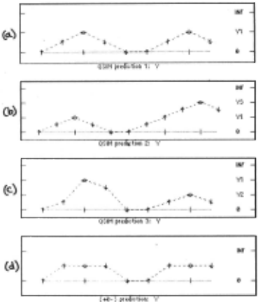
- (a) QSIM prediction 1: the second bounce is the same height as the first.
- (b) QSIM prediction 2: the second bounce is higher than the first.
- (c) QSIM prediction 3: the second bounce is lower than the first.
- (d) {+, 0,-} prediction: the three behaviors are collapsed into a single description.
5 Does Qualitative Simulation Find the Real Behaviors?
Ideally, qualitative simulation will find all and only the actual behaviors of a mPchanism bPing simulated. We take as our "gold standard" the solutiom to tlw ordinary differential !'quation de scribing the mechanism. A qualitativP structure description is less rPstrictive than a cliffcrential <'qnation, so we can expect mul tipll' behaviors produced by the simulation, varying according to factors not captured in the structure description. (For example, if I throw a ball upward with a velocity described only as "posi tive", it might hit the ceiling, or it might not .) First, we want to know that all behaviors that are actually possible arc found by the qualitative simulation. Second, we want to know that every possibility predicted by the qualitative simulation can actually happen.
In QSIM, care has been taken so that the structural descrip tion of a mechanism is an abstraction of its differential equation. The algorithm generates the space of all possible next states of the system givm its current state (Table 1), and each filtering step removes only states which are internally inconsistent. Thus, we prove in detail in [15),
Theorem 1. Each actual behavior of the system is necessar ily amoug those produced by the simulation.
One of the attractive applications of qualitative simulation is to predict possible future states, particularly to warn of sur prising or disastrous events. Although we can trust qualitative simulation to produce every real behavior, the converse is not true: some predictions can be spurious. It is possible for the QSIM algorithm, and local qualitative simulation algorithms in general , to produce behaviors which are not actual behaviors for any physical system satisfying the structural description.
Consider a mass on a spring, oscillating on. a frictionless sur face. The qualitative structural description of this system is
which might also be written in the form of a second-order differ ential equation:
With initial state X(to) = 0, V(to) = Vinit > 0, A(t0 ) = 0, this system is periodic for any function A= -Mlt(X), because if we define total energy as
then equation (2) implies that ftT E = 0.
Starting with X, V, and A equal to 0, Vinit and 0, respec tively, QSIM proceeds straight-forwardly through most of the cycle, predicting a unique successor to each state. Finally, all three parameters approach their initial values. X and A must reach zero together, but there is not enough information to de termine whether V reaches its limit earlier, later, or at the same time.
Figmc 3: QSIM predicts three behaviors for the Spring: one valid and two spurious. The tlm·p columns rcpres<'nt the three behaviors. Look particularly at the qualitative plots for V (the middl<' row).
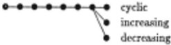
- V and X reach their limits at the same time (the only real possibility).
- X reaches 0 before V reaches Vinit: de creasing oscillation (impossible).
- V reaches Vinit before X reaches 0: in creasing oscillation (impossible).
Figure 4: { +, 0,-} semantics also predicts three behaviors for the Spring: one valid and two spurious. However, we must simulate the initial landmark value of V by defining W(t) = V(t)- Vinit · Compare the qualitative plots for W (the third row) across the three behaviors to distinguish whether V passes its initial value.
- W and X reach zero at the same time (the only real possibility).
- X reaches 0 before W does: decreasing oscillation (impossible). oscillation (impossible) . 3. W reaches 0 before X does: mcreasmg t=
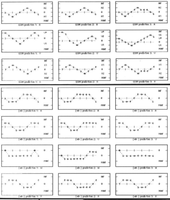
Figure 3 shows how QSlM branches to yield three behaviors rorreo<ponding to increasing, decreasing, and stable oscillation. Figure 4 shows how, using a tramlat<'d variable W to simulate the non-r.ero landmark value Vinit, the same indeterminacy exists under the { +, 0,-} semantics.
As we have seen, only the stable periodic b<'havior is an actual behavior possible for this structural description. Thus,
Theorem 2. There arc behaviors predicted by qualitative simulation which do not correspond to the behavior of any system satisfying the qualitative structure description.
The fundamental problem is that simulation, qualitative or quantitative, is inherently local: the successors to the current state arc computed given only the information in the current state. Given a descriptive framework consisting of the functions and constraints describing the mechanism, and the states to be linked, there is simply not enough information available to elim inate all spurious behaviors.
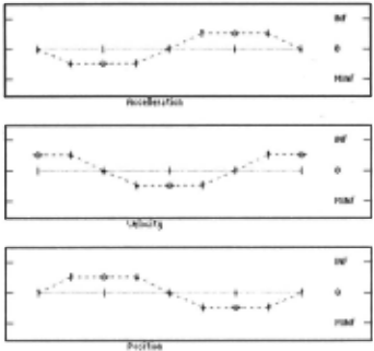
An incorrect solution to this problem is to employ a qualita tive description so coarse that the alternate behaviors arc simply collapsed into a single one. Figure 5 shows the single behavior predicted for the Spring under the { +. 0, -} semantics without an initial landmark value. Precisely like the bouncing ball dis cussed in the previous section, th<' three alternative behaviors are collapsed into a single description, so the problem is not solved, simply inexpressible.
Changing the problem to I><' solv<'d [d<' Klcer, p<'rsonal com nnmirat.ion] ran sometinws avoid t.hi~ <liffirulty in familiar cases. 13y changing the Spring d<'scription to tak<' into account the con· sPrvation of total e1wrgy, an expamkd vi<'W allows QSIM to de termine that there is a single, JWriodic behavior {Figure 6). A physicist can look at equation (2) and recognize or derive the fact that it represents an eucrgy conserving system, aud there fore that the behavior must be periodic. Part of this knowledge is the ability to rc>cognizc the physical system described by a struc ture, and to know that there is a better structural description for it. However, this means that external information is needed to set up the correct problem and reach a useful conclusion in such a case.
These observations yield some important warnings about the proper use of qualitative descriptions of mechanisms, and the result of their simulation.
- The two theorems above have a corollary that highlights their implications for knowledge engineering.
- Corollary. If a structural description is consistent, and if QSIM predicts a single behavior, then that behavior repre sents the actual behavior of the mechanism.
- The structural description must be shown to be consistent, perhaps by demonstrating that it is an abstraction of an ac curate quantitative description, to guarantee that the qual itative simulation will include a genuine behavior.
- If qualitative simulation yields several possible behaviors, further analysis is required before concluding that each rep resents a possible future.
In developing a knowledge base of kidney mechanisms, our Pxpcri(')lce sugg<'sts that th<' most us<'ful knowledge base consists of a collection of lirst.-order vi<'ws, focusin!( on a small portion of tlH' overall mechanism. Each simulation yiPid,; a single behavior, which we therefore know t.o be correct (modulo the assumptions behind the first-order model). .
Thus, much as backward-chaining search provides the math ematical underpinnings for search in a rule-based expert system, so· qualitative simulation may provide the mathematical under piuuings for theory evaluation in a causal reasoning system. If the 1mderpinnings are solid and well-understood, then the se mantics of the kuowledge base is clear, a necessary condition for the creation of powerful reasoning systems.
Acknowledgements
The environment of the MIT LCS Clinical Decision Mak iug Group provides valuable support and stimulation for this research. Christopher Eliot is responsible for the implementa tion of the QSIM algorithm with a very comfortable interface, and for a number of valuable technical contributions. I am also grateful for helpful discussions and observations on qualitative simulation in general and QSIM in particular from Daniel Bo brow, Johan de Kleer, Ken Forbus, Walter Hamscher, Ramesh Patil, Elisha Sacks, Mike Wellman, and Drian Williams.
INF l
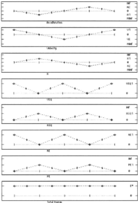
yields a single correct behavior, but requires dornain-spc>cific problem formulation expertise.
@inproceedings{ijcai1985p23,
  title     = {The Limits of Qualitative Simulation},
  author    = {Kuipers, Benjamin},
  booktitle = {Proceedings of the Ninth International Joint Conference on
               Artificial Intelligence, {IJCAI-85}},
  publisher = {International Joint Conferences on Artificial Intelligence},
  editor    = {Aravind Joshi},
  pages     = {128--135},
  year      = {1985},
  note      = {Automated Reasoning},
  url       = {https://ijcai.org/proceedings/1985/23},
}
TY - CPAPER TI - The Limits of Qualitative Simulation AU - Kuipers, Benjamin T2 - Proceedings of the Ninth International Joint Conference on Artificial Intelligence, IJCAI-85 PB - International Joint Conferences on Artificial Intelligence PY - 1985 SP - 128 EP - 135 UR - https://ijcai.org/proceedings/1985/23 ER -Copied
Machine-readable versions of this paper, for tools and AI agents:





