
Recurrent Neural Networks for Sequence Production
Proceedings of the Thirteenth International Joint Conference on Artificial Intelligence. Machine Learning. Pages 1114-1118.
© 1993 International Joint Conferences on Artificial Intelligence
Abstract
In an empirical study, simple recurrent networks (SRN s, Elman, 1990) and recurrent cascade correlation networks (RCC, Fahlman, 1991) are compared with respect to a sequence production task. The application system that includes these networks extracts relevant information from incoming e-mail messages during a training period, learns the reaction to the incoming message, i.e., a sequence of user actions, and uses the learned representation for the proposal and preparation of user reactions. The performance of both network architectures in terms of network size and learning speed for a given data set is examined. Our results show that (1) RCC generates smaller networks with better performance compared to SRNs and (2) learns significantly faster than SRNs.
- Diederich, J.; Thuemmel, A.; Bartels, E.: Recurrent and Feedforward Networks for Human-Computer Interaction. In: Neumann, B. (Ed.): ECAI-92, lOth European Conference on Artificial Intelligence. Chichester: John Wiley & Sons 1992, 206-207
- Elman, J .L.: Finding Structure in Time. Cognitive Science 14 (1990) 179-211
- Fahlman, S.E.: The Recurrent Cascade-Correlation Architecture. Pittsburgh, Penn.: Carnegie-Mellon University (CMU), May 1991 = CMU-CS-91-110
- Jordan, M.L. : Attractor dynamics and parallelism in a connectionist sequential machine. Proc. of the 8th conference of the Cognitive Science Society 1986.
- Hillsdale, N.J: LEA 1986. Reprinted in: Diederich, J. (Ed.): Artificial Neural Networks: Concept Learn- ing. IEEE Computer Society Neural Network Tech- nology Series, 112-127, Los Alamitos, Ca. 1990
- Yang, J. & Honavar, V.: Experiments with the Cascade-Correlation Algorithm. Dep. of Computer Sciencs, Iowa State University, lA, USA., 1991 = Tech. Report #91-16
References were extracted automatically from the PDF and may contain errors.
Full text extracted automatically from the PDF; figures, tables and equations may differ. The PDF is the version of record.
1 Introduction
In this paper, a comparison of two recurrent network architectures is presented. The performance of sim ple recurrent networks (SRN, Elman 1990) is compared to the recurrent cascade correlation architecture (RCC, Fahlman 1991). For both architectures, this study fo cuses on the required network size (number of hidden units) and the speed of the learning process to perform a given task.
The background is a neural network application (called NECAS), an advanced mail tool which runs on top of UNIX mail. Here, relevant information from in coming messages is extracted and neural networks learn user actions in response to these messages. In Diederich et al. (1992) it is shown that SRNs are capable of learn ing this task. A problem with SRNs is that the size of the network (number of hidden units and layers) has to be chosen in advance, which may lead to inappropriate choices (e g., to many hidden units) and consequently to bad generalization.
RCC, however, incorporates an incremental learning
Recurrent Neural Networks for Sequence Production
Joachim Diederich* Markus Wasserschaff**
*Neurocomputing Research Centre School of Computing Science Faculty of Information Technology Queensland University of Technology GPO Box 2434
Brisbane Q 4001 Australia
**German National Research Center for Computer Science (GMD) Institute for Applied Information Processing (FIT) P.O. Box 1316
D-5205 St. Augustin 1 Germany
algorithm and is supposed to build reasonable small networks. The size of the generated RCC-network gives an indication of a reasonable size for a SRN.
In this comparison, a sequence production process is examined. More precisely: The relation between a pattern's position inside a sequence and the difficulty (i.e. number of pattern presentations) to learn it, is investigated.
Our objectives are the following:
- Optimization of the size of the SRN using the results of the RCC experiments
- Comparison of the performance of RCC vs. SRN with respect to our applications data set
- Study the performance of the networks doing se quence production. For instance, we are inter ested in the following question: Given a sequence of training patterns and a recurrent network: Is there a relation between a patterns position in side a sequence and the difficulty (i.e., number of pattern presentations) to learn it?
In this paper, we first give an introduction to SRNs. Next, the particular networks we are using (called NECAS Recurrent Network; NECAS RN) plus the RCC-architecture is described. Section 3 provides an overview of the data set used for experimental purposes. Next, in section 4, the methodology used for evaluation is outlined and after the presentation and discussion of the results in section 5, we conclude with some remarks on future work.
2 The neural network architec tures
2.1 Simple recurrent networks
A simple recurrent network for sequence production can emulate a finite-state machine and implements an out put function f and a next-state function g. At each moment in time, an action is chosen based on the cur rent state s, and the state is then updated to allow the next action to be chosen (Jordan, 1990, p.115). The function f determines the output action 2n at time n,
and a function g determines the state ·n+l,
where both functions depend on the constant plan vector p as well as on the current state vector ·n. In a Jordan-Network (Jordan 1986, 1990), "plans," "states" and" actions" are distributed patterns of activation over separate groups of units. All feedforward connections implement f and all recurrent connections implement g. The plan units and the state units are the input units. The network takes a plan as input, i.e., a distributed pattern of activation over the plan units, and produces a sequence of actions over the output units.
The Jordan-networks have full connectivity between input , hidden and output layer and one-to-one connec tivity from the hidden or output units to the linear state units. Feedback links have a fixed weight (1.0) and their sole purpose is to copy a hidden or output unit activa tion pattern to the state units. In other words, the activation pattern over the state units at time step t equals the hidden or output unit activation pattern at t -1.
A modification of this approach leads to Elman networks: (The) network i· augmented at _the inpu~ level by additional unit.; call(ed) contezt unat. (prevaou·ly called .tate unit.). The·e unit. are al·o "hidden" in the ·en·e that they interact ezclu1ively with other node~ internal to the network, and not the out.ide world (El man, 1989).
The activation patterns of the hidden units at time step t are copied onto the context units and presented with the input at the next time step (see Figure 1): Thu·, the hidden unit· have the ta1k of mapping both an ezternal input, and al·o the previoUI internal ·tate of 1ome de·ired output. Becau·e the pattern· on the hid den unit. are 1aved a· contezt, the hidden unit· mu.t accompli·h thi· mapping and at the ·ame time develop repre·entation· which are u·eful encoding· of the tempo ral propertie· of the ·equential input. Thu·, the internal repre1entation· that develop are 1en1itive to temporal contezt; the effect of time i· implicit in thue internal 1tatu (Elman, 1989).
2.2 The NECAS recurrent network
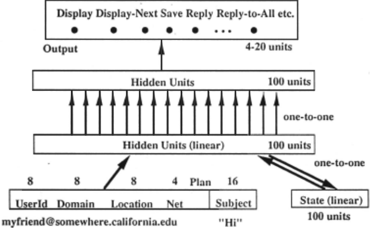
The architecture of the recurrent network used in our application is similar to simple Elman-networks. It uses two hidden layers and copy-back links from the first hidden layer to the state units (similar to Elman Networks). The first hidden layer units, the state units plus the output units are all linear units. There is full connectivity in feedforward direction, but fixed one-to one connections are used between the first and second hidden layer. Also, there is fixed one-to-one connectiv ity between the first hidden layer and the state units.
The use of linear units as part of the first hidden layer allows to preserve input information and to copy the hidden unit activation to the state units before the outputs are squashed by the sigmoidal output function. Without this additional hidden layer, it was not possi ble during learning to reduce the sum-squared error to a minimum.
The input layer (i.e., the plan units of the NECAS recurrent network) consists of sets of units which repre sent information from the incoming message (see Figure 1). In detail, there are 8 units for the representation of the account name, 8 units for the coding of the domain, (for instance "cs"), 8 units for the representation of the location (such as "berkeley") and 4 units for the cod ing of the network (for instance "edu" as part of the Arpa net). Due to the binary input coding, we use 8 bits for the representation of the account name, domain and location and 4 bits for the coding of the network. Furthermore, we currently use 16 units for the represen tation of the subject (the first non-function word in the subject line is used). A random bit vector represents an individual account name, location, network etc.; it is guaranteed that a bit vector is used only once in the training and test set. The random bit vectors are re trieved from hash tables that are used and updated by the NECAS system. New random bit vectors are gen erated, stored and used when new information comes m.
Note that we use the recurrent network for sequence production and that the network starts with random initial weights. Due to the fixed plan vector, the net work has to use the state information to adjust weights. This training task is difficult, in particular during early periods of the training due to the erroneous activation patterns over the state units. Therefore, the network must have a significant number of hidden layer and state units.
The initial experiments were done with a varying sizes of the input and output layer ( 44-56 units for ac count name, domain, location, network and subject in the input layer and 4 or 20 units in the output layer) . Good ·results are reported from experiments with the following configuration: first and second hidden layer as well as the group of state units have 100 units each, the output layer contains 20 units and the plan is a 44 bit vector (Diederich et al., 1992).
2.3 The recurrent cascade correlation architecture
Fahlman (1991) introduced the Recurrent Cascade Cor relation Architecture (RCC). Instead of only adjusting the weights of a fixed network topology, the idea is to start with a minimal network and to add hidden units as necessary.
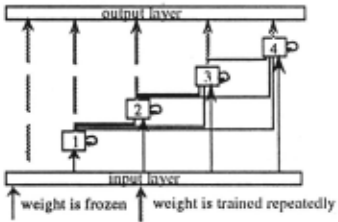
So the initial network starts with no hidden units, and only the weights to the outputs are trained. If this is not satisfying, a new hidden unit has to be added.
The learning and network construction process works as follows: The algorithm starts with a set of new units, called candidate pool. These units have ran domly initialized, weighted connections from the input nodes and all the hidden units already present in the network. At that time their outputs are unconnected. Then, their incoming links are trained on the training set and adjusted in order to maximize the correlation between the candidates outputs and the remaining error (Fahlman, 1991). When there is no improvement, this process stops and the candidate with the best "correla tion score" is added permanently. Its weights are frozen now, which means that this node becomes a new unique feature detector in the network. In order to integrate this new hidden unit, the weights of the output layer are trained for multiple epoches (Fahlman, 1991). This scheme of adding hidden units and retraining the out put layers weights is repeated until success (when the error falls below a predefined threshold or no bit er rors are found) or a maximum number of hidden units is reached (which means failure). Fahlman points out that this learning algorithm works like a greedy algo rithm because the network is extended stepwise until a solution is found.
Note that every new hidden unit adds a new hidden layer to the network, because it is connected to all pre vious hidden units. Recurrence is achieved by adding self-recurrent links to all hidden units. So at time step t + 1 the activation of time step t is fed back to the hidden unit. Such a constructive learning algorithm is expected to build a near minimal network for a given problem, because every hidden unit serves as a unique feature detector, and no a priori and maybe inappro priate guesses about the size of hidden layers have to me made.
In our experiments, we used the same coding for the inputs and outputs as for the NECAS RNs in section 2.1.
2.4 The data set
We use artificially generated and natural data (ex tracted by observing real users) for training and test purposes. The artificial training set is used for evalua tion purposes, in order to test various network architec tures. Also, because of the size of the NECAS recurrent network, training has to be done with sufficiently large training sets.
An artificial training set was constructed by extract ing addresses from the Usenet and defining a number of explicit rules for typical user responses. These rules are used to generate an artificial data set. Six of these rules are "useful heuristics"; two are response patterns to in dividual senders. The rules encode response tendencies that a real e-mail user might have.
For example, a "useful heuristic" is that messages from sender at well-known research labs and universi ties are more important than messages from unknown locations. Therefore, the hypothetical user, who is sim ulated by the artificial data set, responses with long se quences of e-mail actions to messages from "important"
| Rule | Number of Sequences | Length (no. of patterns) |
|---|---|---|
| 1 | 25 | 2 |
| 2 | 25 | 2 |
| 3 | 50 | 6 |
| 4 | 75 | 4 |
| 5 | 100 | 4 |
| 6 | 75 | 5 |
| 7 | 50 | 6 |
| 8 | 25 | 2 |
| 9 | 75 | 3 |
| Position i = | # of pattern at position i |
|---|---|
| 1 | 500 |
| 2 | 500 |
| 3 | 425 |
| 4 | 350 |
| 5 | 175 |
| 6 | 100 |
locations. 550 sequences with a total of 2050 input output patterns were generated by use of these rules. The length of an individual sequence ranged from two to six patterns (the end of a sequence was indicated by a special marker).
The following two rules are examples for the type of rules used to generate the artificial training set:
- If a message comes from the location "berkeley," then "display" the message, "save" the message and "reply" to the message.
- If a message comes from an "administration" (do main) at the location "berkeley," then "display" the message, "save" the message, "save the mes sage in a special folder" and "reply" to the mes sage.
Table 1 shows the structure of the training set. We also counted the number of training patterns that oc curred in a certain position inside of a sequence (Table 2).
3 The evaluation method
An important question is: How large will the RCC network be, giv:en the same data set as for the fixed NECAS RN? In order to answer this question, we used the following method: First, we run RCC on the data set until the error was significantly reduced (we assume a rms-error 1 below 0.1 indicates success) and record the number of hidden units. We built up a NECAS RN with the same number of hidden units and train the network as well. Because RCC has the advantage of shortcuts from inputs to outputs, we have repeated the training session with a modified NECAS RN, where shortcuts from inputs to outputs are part of the network. In an additional experiment, we replaced the linear activation functions of the outputs with sigmoidal functions.
For RCC we used sigmoid unit types (standard range from 0.0 to 1.0), and a sigmoid prime offset of 0.1. The RNs were trained with a small learning rate (0.0005) , a momentum of 0.9 or no momentum and a negative bias ( -2.5).
Another objective is the evaluation of the sequence production process. Therefore, we use a special kind of error report for all experiments. First we divide the data set p into six sets Pt, .. , 1'8· Pi contains all the training patterns which appear in their sequences at position i. Then for each epoch we sum up the squared error for all pattern in Pi, averaged over the size of Pi , resulting in a position error ei
where OJJ(P) is the activation of output lc for pattern p, tl(P) is the corresponding teaching input and n is the number of output units. This position error allows to show how good the network performs on sequence production.
4 Results
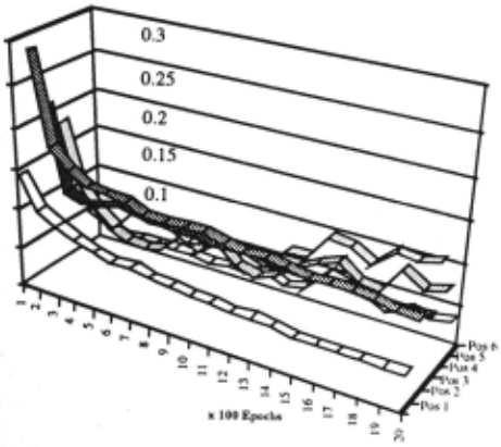
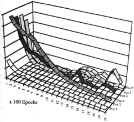
RCC was able to learn the artificial data set in about 4300 epoches. The error decreased continuously as new hidden units were added. The behavior of the NECAS RNs were different. In general, the rms-error was re duced very fast to 0.3, but got stuck above 0.2. A rms-error of 0.26, as computed for one NECAS RN, means a total of 304 output bit errors 2 over the whole training set. For the RCC network, we counted 31 bit errors after completion of the training. Figure 5 shows that NECAS RNs with linear outputs give slightly bet ter results than networks with sigmoidal outputs. An important detail is that there is only a small differ ence in performance if shortcuts from inputs to outputs are used. One should expect that networks with these shortcuts are more powerful, so the interpretation is that 43 hidden units are not sufficient. Because we got good results with 100 hidden units (our initial guess),
1 The rms-error is defined by
2 An output is counted as erroneous, if its activation de viates from the teaching input by more than 0.3.
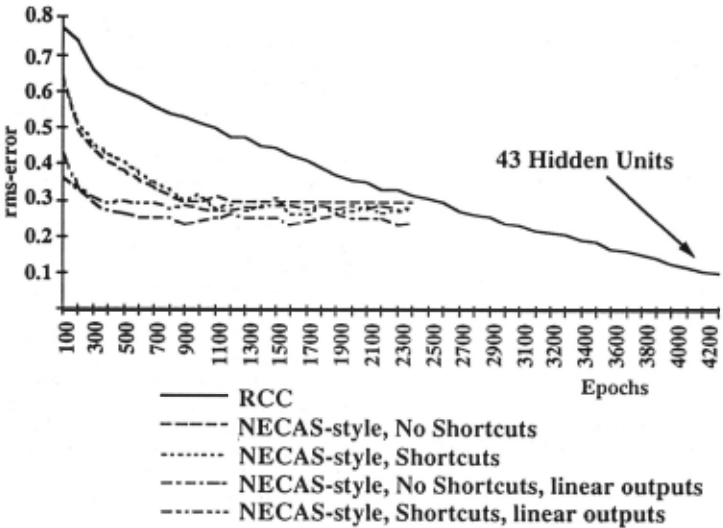
we expect that the optimal SRN for our data set must have about 100 hidden units.
In summary: RCC is able to build up smaller net works compared to the SRNs we tested. Even though more training epoches are necessary, RCC was faster, for the following reasons:
- In backpropagation, each presentation of a train ing case requires a forward pass and a backward pass through all layers in the network. RCC can train single layers.
- In RCC, many training epoches run while the net. work is small compared to its final size.
In our simulations, RCC required ten times less compu tation time than the NECAS RN, for the same number of epoches.
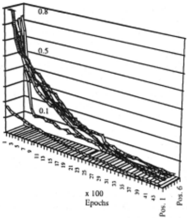
Figure 4 to 6 show the position errors for the com pared networks. At the first glance these results are very unexpected. A first assumption is that the error increases with the length of a sequence. But while the error for patterns in the first and the last position is de creased rapidly, the error for the other positions is only slowly reduced. The reason is the structure of the data set. Only 18.1% of all sequences have the maximum length of six patterns. But there are 325 "medium sized" sequences (that is: 2-4 patterns) which were gen erated using six rules. This means that the major part of the data set consists of short sequences distributed over many classes.
~·
Figure 6: Position error for a NECAS RN with 43 hid den units, shortcuts from inputs to outputs and sigmoid output units.
5 Discussion
To find the right structure and size of a neural network is often difficult and a non-trivial task. Automating this process using incremental algorithms (in our case RCC) is an alternative. Our experiments are a first attempt to determine the effectiveness of RCC in comparison to SRNs on a real-world problem. Our results show that RCC is more efficient. Of particular interest for our application is the ability to generalize from unknown or noisy data. This will definitely be the next step for future research. Even though Fahlman (Fahlman, 1991) reports superior generalization for his benchmark tests, we will have to verify this for our own data set (for the non-recurrent version CCA there exist results that neglect the superiority (Yang & Honavar, 1991)). Another weak point of RCC is the lack of a theoreti cal model for this architecture and the large number of parameters that control RCC (and often their choice is left to intuition).
6 Acknowledgments
The architecture of the NECAS recurrent network is partially based on suggestions by Andreas Weigend. The use of artificial data sets for test purposes was sug gested by David Rumelhart . We would like to thank C. Doherty for making the code for the RCC simulator available.
@inproceedings{ijcai1993p154,
  title     = {Recurrent Neural Networks for Sequence Production},
  author    = {Diederich, Joachim and Wasserschaff, Markus},
  booktitle = {Proceedings of the Thirteenth International Joint Conference on
               Artificial Intelligence, {IJCAI-93}},
  publisher = {International Joint Conferences on Artificial Intelligence},
  editor    = {Ruzena Bajcsy},
  pages     = {1114--1118},
  year      = {1993},
  note      = {Machine Learning},
  url       = {https://ijcai.org/proceedings/1993/154},
}
TY - CPAPER TI - Recurrent Neural Networks for Sequence Production AU - Diederich, Joachim AU - Wasserschaff, Markus T2 - Proceedings of the Thirteenth International Joint Conference on Artificial Intelligence, IJCAI-93 PB - International Joint Conferences on Artificial Intelligence PY - 1993 SP - 1114 EP - 1118 UR - https://ijcai.org/proceedings/1993/154 ER -Copied
Machine-readable versions of this paper, for tools and AI agents:





