
Learning Finite Automata Using Local Distinguishing Experiments
Proceedings of the Thirteenth International Joint Conference on Artificial Intelligence. Machine Learning. Pages 1088-1092.
© 1993 International Joint Conferences on Artificial Intelligence
Abstract
One of the open problems listed in [Rivest and Schapire, 1989] is whether and how that the copies of L • in their algorithm can be combined into one for better performance. This paper describes an algorithm called v· that does that combination. The idea is to represent the states of the learned model using observable symbols as well as hidden symbols that are constructed during learning. These hidden symbols are created to reflect the distinct behaviors of the model states . The distinct behaviors are represented as local distinguishing experiments (LDEs) (not to be confused with global distinguishing sequences), and these LDEs are created when the learner's prediction mismatches the actual observation from the unknown machine. To synchronize the model with the environment, these LDEs can also be concatenated to form a homing sequence. It can be shown that v· can learn, with probability 1 - e' a model that is an {-approximation of the unknown machine, in a numb er of actions polynomial in the size of the environment and ~(logi)
- Execute h; a.nd construct Ps(so, h;) a.nd Os(r, hi);
- D. Angluin. Learning regular sets from queries and counter-examples. Information and Com- putation, 75(2), November 1987.
- [Rivest and Schapire, 1989] R. Rivest and R. Schapire. Inference of finite automata using homing sequences. In Proceedings of 21th Annual ACM Symposium on Theory of Computing, 1989.
- [Rivest and Schapire, 1993] R . Rivest and R . Schapire. Inference of finite automata using homing sequences. Information and Computation (to appear), 1993.
- [Shen, 1989] W . Shen . Learning from the Environment Based on Actions and Percepts. PhD thesis, Carnegie Mellon University, 1989.
- [Shen, 1993a] W. Shen. Autonomous Learning from the Environment. W .H. Freeman, Computer Science Press, Forthcoming 1993.
- [Shen, 1993b] W. Shen. Discovery as autonomous learn- ing from the environment. Machine Learning, 10, 1993.
- [Utgoff, 1986] P. Utgoff. Machine Learning of Inductive Bias. Kluwer Academic, 1986.
References were extracted automatically from the PDF and may contain errors.
Full text extracted automatically from the PDF; figures, tables and equations may differ. The PDF is the version of record.
1 Introduction
Learning deterministic finite automata is an interesting topic for many research areas. It relates to language learning, autonomous systems, constructive concept in duction, and perception with hidden states. There are two basic problems that underlie the task: the construc tion problem and the synchronization problem. The for mer is a problem of how to construct a perfect model of the unknown machine based on the feedback of actions, and the latter is a problem of how to synchronize the model with the unknown machine. An existing solution to the construction problem is the L · algorithm devel oped by [Angluin, 1987] . U can learn regular expres sions using membership queries and equivalence queries but it requires a means to reset the unknown automa ton to a fixed state for synchronization. The algorith m developed by [Rivest and Schapire, 1989] extends U to deal with the synchronization problem by learning a homing sequence of the unknown machine. However, for each different output of the current homing sequence, they create an independent copy of L ·. Every time the homing sequence is updated, all (or some of) the copies of L · are discarded. It is an open question whether and how that the copies of L · can be combined into one.
This paper describes the v· algorithm that solves both the construction problem and the synchronization problem using a single mechanism: local distinguishing experiments (LDE). Since LDEs are incrementally dis covered through the interactions with the environment and can be used to construct both hidden states and homing sequences, there is no need for keeping sepa rate copies of models or discarding the models when new LDEs are discovered.
2 The Basic Definitions
Learning deterministic finite automata can be viewed as a special type of learning from the environment [Shen, 1989; Shen, 1993a]. The task of the learner is to con struct an exact model of the environment to predic t the consequences of its actions. Here the environ ment E is defined as a variation of a Moore machine (A , Z,Q,6,p,r), where:
- A is a finite set of input symbols;
- Z is a finite set of output symbols;
- Q is a finite set of environmental states;
- 6 : Q x A --+ Q is the transition function of E ;
- p : Q --+ Z is the appearance function of E;
- r is the current state of E. When an input symbol a E A is received by E, r is updated to be 6(r, a) . Initially, r can be any state in Q.
We assume E is strongly connected. We say that E is transparent if its p is one-to-one, and E is translucent if its p is many-to-one.
A model M of the environment E is defined as (A, Z, S, </>, t), where:
- A is a set of actions of the learner;
- Z is a set of percepts of the learner;
- S is a set of model states represented as Z{O, 1}i, where {0, 1}; is a finite sequence of binary symbols constructed by the learner;
- 4> : S x A --+ S is the transition function of M;
- t is the current model state of M. When an action a E A is applied to M, t is updated to be 4>(t, a).
Model states are described by expressions 8 = z{O, 1}., where z E Z. A description 8 represents a set of model states whose prefix is s. For example, z1 represents all the model states whose prefixes are z1, and z10 represents all the model states whose prefixes are z10. Clearly, z10 is a subset of zl. Notice that the symbol "s" is used to denote both a set of model states and a single model state (when the set is a singleton). From the context, this uniform representation of model state(s) should not cause any confusion.
Given a descriptions = z{O, 1 }*,we use o(s) to denote the observed part of s, and f3(s) for the constructed part of s. For example, if s = z0110, then o(s) = z and P(s) = 0110.
We denote the set of all finitely long action sequences by B = A·, and use 6(q, b), where b E B, to denote the environmental state reached by executing sequence b from an environmental state q. This denotation is also applicable to M's transition function 4>.
In the process of learning, we allow the function 4>( s, b) to be nondeterministic. That is, the value s' = 4>( s, b) may represent a set of model states whose prefix is s'. In that case, 4>( s, b) denotes the set of model states, s', reachable by executing the action sequence b from the model states. As a special case, if 4>(s, b) does not exist, we write 4>(s, b) =?. The symbol "?" represents the entire set of model states.
We say that a single model state s is visibly equivalent to an environmental state q if p(q) = o(s) . Furthermore, we say that M is perfect and synchronized with respect to E if the current model state t is visibly equivalent to the current environmental state r, and for all sequences of actions b E B, the model state 4>( t, b) is also visibly equivalent to the environmental state 6( r, b). Our objec tive is to learn a perfect and synchronized model of the environment.
Let r be the current environmental state. We refer to the sequence of percepts obser·ved in the environmental states visited by executing b = aoa1 ... a. from r as the observation sequence of b from r, denoted as:
We assume that the environment is reduced: for every pair of unequal environmental states q1 and q2 , there is an action sequence b such that OS(q1 ,b) :f OS(q2,b).
Somewhat parallel to an observation sequence of b from r, we define the prediction sequence of b at t to be the sequence of model states visited by executing actions b = aoat ... a. from the current model state t, denoted as:
Before we define local distinguishing experiments, let us first consider an example. Suppose you are to predict (not actually doing it) whether you can lift some boxes. These boxes look identical from the outside. However, if you open the lid you can see that a box is either empty or containing some weight that is too heavy for you to lift . Naturally, in order to make a correct prediction, all you need to do is open the lid and see inside. The sequence of "open-lid" and "see-inside" is a local distin guishing experiment. It uses your actions and percepts to reveal more information about a particular environ mental state.
Formally, let z be the current observation p(r) from the environment (seeing a box), and 8 = zc, where cis a binary string, be a set of model states (the box is either empty or too heavy) that contains the current model state t (the true status of the box). Notice that the necessary condition for s to contain tis that o(s) = a(t). We refer to a set of relations that can reduce the set zc to either zcO or zcl, whichever contains t, as a local distinguishing experiment of zc, denoted as LDE(zc?):
where b is a sequence of actions, [x] = OS(q1 , b) and [y] = OS(q2, b) are two different previous observation sequences of a from some environmental states q1 and q2 whose appearance are z (i.e., p(qt) = p(q2 ) = z), and b, [x], [y], and the current environmental state r, satisfy the relation :
Thus, if it is known that the current model state t is in zc (e.g., a box is either empty or too heavy), then one can determine if t is in zcO or zcl by executing b (e.g., opening the lid) in the current environmental state r , comparing the actual observation sequence (e.g., what you see inside the box) with [x] and [y], and concluding either t was in zcO or t was in zcl. We define the length of LDE(zc?) to be the length of its actions b.
3 The Construction and Synchronization Problems
It is interesting that when the environment is transpar ent, the construction and the synchronization problems can be solved easily. Since all the transparent environ mental states are visibly different, we can treat q = z. The synchronization problem is trivial because what we see is where we are. Thus, we can build 4>(z, a) from a state z by simply executing a and observe the state reached. If 4>(z, a) is already known for every action in A, then either we can find a path based on what is al ready known about 4> to a state for which this not the case, or we have finished learning a perfect model of E. Figure 1 gives this simple algorithm in detail. For con venience, we will refer to this algorithm as D algorithm.
In general, however, environments are not transpar ent. Because the appearance function p is many-to-one, two or more environmental (and model) states may have the same output and the learner's current observation may not uniquely determine what the current environ mental (and model) state is. For example, in the SHAPE environment (copied from [Rivest and Schapire, 1989]) shown in Figure 2, there are two actions, x and y, and four environmental states I, II, III, and IV. A learner, however, can only see the two shapes of the nodes: 0 or
- Initializing S = Z and t/1 = {} .
- Repeat
- Let the current model state t = zo, where zo = p(r) is the current observation from the environment;
- Select actions ba such that 1/1( 1/1( t, b), a) does not exist;
- Execute ba;
- Record OS(r, ba) = [zo, ... , zl"l· za];
- Insert t/l(zlbl> a)= Za into 1/1;
- Until t/l(z,a) exists for all z E Z and a EA.
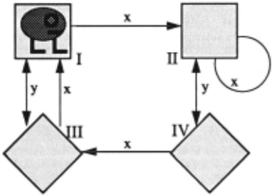
Figure 2: The SHAPE environment
0. When D is seen, the learner does not have enough information to determine whether the current environ mental state is I or II.
To model a translucent environment, model states must consist of both observed symbols and constructed symbols in order to distinguish different environmental states that appear alike. For example, one way to model the states in the SHAPE environment is to use one hid den binary symbol for the model states. So, one can use DO for state I, D1 for state II, 00 for state III, and 01 for state IV.
Because of the hidden symbols involved in the mod el states, both the construction problem and the syn chronization problem become substantial. In particular, since the number of model states is greater than the number of percepts, the learner must determine when and how to construct new model states. Since there are more than one model states whose observed part matches the current observation, the learner must also determine which model state is current. Clearly, the simple D al gorithm must be extended to deal with these problems.
4 Model Construction with LDEs
To solve the construction problem, we use a technique called surprise-identify-split [Shen, 1989; Shen, 1993a]. The main idea is that the learner always predicts the con sequence of its action based on the model that is learned. Whenever the actual consequence does not match the predicted consequence (a surprise), the learner identifies a "faulty" state in the model that is responsible for the surprise and splits that state into two by appending to it a new binary symbol. The action sequence that causes the surprise, along with the prediction sequence and the observation sequence at that time, is defined as a new LDE for distinguishing the two new states in the future.
4.1 Surprises
Let r be the current environmental state (which is un known to the learner), z0 = p(r) be the current ob servation, and so be the current model state, where o(s0) = z0 . Then, after executing a sequence of ac tions b = a0a1 ... a., we have a prediction sequence and observation sequence as follows:
We say that there is a surprise if the latest prediction is visibly different from the latest observation: Ze+l :f o(se+d·
For example, suppose a learner in the SHAPE environ ment has learned, using the D algorithm, the following model:
and suppose that the current environmental state is III (which is unknown to the learner), and the learner's cur rent observation is 0. Since the learner thinks that the current model state is 0, the prediction sequence and the observation sequence of executing the action z are:
There is a surprise in the above prediction/observation sequences because their last elements are visibly differ ent: 0 :f D.
4.2 Identify and Split
Since the learner's predictions are based on previous ob servations, a surprise means that some model state is mistakenly representing more than one environmental s tate. The learner must identify such a "faulty" model state, and split it into two new model states: one repre sents the prediction, the other represents the surprising observation.
The process of identify and split is simple when the surprise is the first one (i.e., there is no previously de fined LDEs) . In this case, the state Be in PS(so, b) (see Equation 1) is the "faulty" state. This is because Be is the state to which the same action, a., causes different consequences, se+l and Ze+l· Thus, s. is split into BeO and s.1 and a LDE for s. is defined:
For example, in the above surprise between PS(O, z) and OS(III,z), the faulty model state is 0 and it is split into 00 and 01, and a new LDE is defined as:
When the surprise is not the first one, then the pro cess of identify and split is more complex. In this case, since there exist previously defined LDEs, the elements in PS(s0 , b) (see Equation 1) and OS(r, b) (see Equa tion 2) may represent sets of model (environmental) s tates. Before the faulty state can be identified, these elements must be "refined" (i.e., reducing the number of model states each element represents) using the existing LDEs. In fact, such a refinement is conducted every time the prediction/observation sequences are extended (i.e., a new action-observation pair becomes available).
The refinement of the prediction sequence is accom plished as follows. Let
be the refined sequence of PS(s0 , b). By definition, the relation between PS(so, b) and Ps(so, b) is that p; ~ s; for all 0 < i < e+ 1. Initially, each p; is copied from the correspo~ding s; in the prediction sequence P S( s0 , b), except when s; =? (i.e., no prediction for this particular step), p; is copied from z; in the observation sequence OS(r,b). Then, for each p; in Ps(s0 ,b) from the end to the beginning, we repeatedly check if it can be "shrunk" by some existing LDEs. In other words, for each p;, we check if there exists a LDE(p;?) = (l;p;O, [x];p;1, [y]) such that I is equal to a subsequence of b that begins with a;, say I= a; ... aj, and [x] (or [y]) is equal to the subsequence z;, ... , Zj+l in OS(r, b). If so, p; is set to be p;O (or p;1). The same procedure is also used to refine the observation sequence OS(r, b) to get:
where o; ~ z; for all 0 ~ i ~ e+1.
To illustrate the refinement procedure, suppose that the learner's current model of the SHAPE environment is M1 (we will show how M 1 is built from Mo shortly):
and the current prediction sequence and observation se quence are:
Initially, Ps(O,yx) = [0,0?,0] and Os(II,yx) [0, 0, 0]. Notice that the third element of Ps(O, yx) is copied from 0 S( II, yx) because the corresponding pre diction in PS(O, yx) is a "?." Then, using the existing LDEs, we refine these sequences to get:
Notice that the second elements in Ps(O, yx) and Os(II,yx) are inferred by the existing LDE(O?) = (z; 00, [00]; 01, [00]), defined in Equation 4, respec tively.
Once PS and OS are refined to be Ps and Os, we are ready to identify the faulty state. The faulty state is the state PI< in Ps(s0 , b), where k is the greatest index such that PI< ~ o~c and Pl<+l f/, OJc+l· The motivation is that PI< is the state to which applying the same action yields different next states. It can be shown that such PI< always exists when a surprise occurs. However, it is still a open question whether PI< is always the "optimal" faulty state to split. When PI< is not optimal, the states created by splitting PI< may become wasted: they become unreachable eventually.
After PI< is identified, it is split into p~cO and PI< 1, and a new local distinguishing experiment for PI< is defined as follows:
Notice that Equation 7 is a generalized version of E quation 3. Notice also that the length of the new LDE (because of the way PI< is identified) is at most one plus the maximum length of the existing LDEs.
In the SHAPE environment example, after Ps(O, yx) and Os(II, yx) are computed, the state 0 is identified to be faulty, and it is split into DO and Dl. A new local distinguishing experiment LDE(D) is defined as:
4.3 Model Refinement
Models are refined in two occasions: when the refined prediction sequence is more deterministic than the mod el, and when a new LDE is defined after a surprise.
In the first case, since a refined prediction sequence incorporates the most recent observations from the en vironment, it may contain information that is not in the current model. Such information provides opportunities to update the model accordingly. For example, from Ps(D, yx) we can upgrade the nondeterministic tran sition <f>(D, y) = 0? in M1 to </>(D, y) = 00, and the updated M1 is:
In general, the transition function is updated accord ing to Ps as follows. If there exists p;, a; and Pi+l, such that p; is a single model state and Pi+l is a subset of <f>(p;, a;), then <f>(p;, a;) is set to be Pi+l·
In the second case, after the model state Pk is split, the transition function 4> is modified as follows: ( 1) delete the obsolete transitions <f>(Pk, ·) from </> since Pk is no longer a single model state; {2) insert two new transitions <f>(p~cO, ak) = Pi+l and <f>(p~c1, a~c) = Oj+l into</>. Notice that all the transitions that go into p;, i.e., </>{·, ·) = p;, now become nondeterministic {since PI< now represents two model states p;O and p; 1 ). Such non determinism will be resolved in future explorations by model refinement in the first case.
An example of model refinement after a surprise is how M1 is built from M0 · When the state 0 is split in Procedure D*(A, Z):
- Initialize S = Z, ¢J = {}, and t =?;
- Repeat 2. While t is a not single model state, dot -GOTO-A-M-STATE{); 3. Let r be the unknown current environmental state; 4. Select actions b = b'a such that ¢(¢{t, b'), a)= p and p is not a single model state; 5. 6. 7. If b is empty, then b - random action sequence, else b = b ·I where lis the actions in LDE(p?); For each action ai in b = ao,aJ, ... ,aj, ... ,ajbl· do: 8. Execute aj, construct PS(t , ao ... aj), OS(r, ao ... aj), 9. Compute Ps(t,ao ... ai) = [po, ... ,pj,Pi+d and Os(r, ao ... aj) = [oo, ... , Oj, Oj+d, 10. Refine the model M (See case 1 in Section 4.3); 11. If a(si+d :/: Zj+l (a surprise), then 12. call ID-SP-RE{Ps, Os); 13. Goto 1; 14. Until no surprises for at least n actions.
Procedure ID-SP-RE(Ps(t, b), Os(r, b)): Let k be the greatest index in Ps(t,b) such that Pic~ o1c, Plc+l S?; Olc+li Replace PI< in S by p,.O and p,.l; Define LDE(p,. ?) (See Equation 7) ; Refine the model M (See case 2 in Section 4.3).model M0 after the first surprise (see Equation 4), we get model M1 according to the above refinement steps. (The readers can verify that .) Similarly, when the state D is split after the second surprise (see Equation 8), the model M~ becomes a new model:
5 The D* Algorithm
With the techniques described in Section 4, we now present the D* algorithm in Figure 3. For the moment, we assume that a solution for the synchronization prob lem is given as a procedure "GOTO-A-M-STATE" which tells the learner what the current model state is.
It is obvious that the D* algorithm is an extension of the simple D algorithm. Line 2 determines the curren t model state t using the assumed procedure GOTO A-M-STATE. Lines 4 to 6 select actions. Similar to the D algorithm where actions are selected for con structing nonexisting transitions, n· selects actions to reduce the nondeterminism (nonexistence is a special case) of transitions. To reduce the nondeterminism of ~(~(t, b'), a)= p, we use LDE(p?) and run its actions I after b' a (Line 6). If the current transition ~ is already both complete (i.e., ~(s, b) exists for all s E Sand bE B) and deterministic, then a sequence of random actions is selected at Line 5. The purpose of random actions is to look for surprises (or counterexamples) . Clearly, if an oracle were available to provide such counterexamples, then line 5 will be the place to call the oracle.
For each action in the select action sequence, Lines 8 and 9 construct and refine the prediction and obser vation sequences (Section 4.2), and Line 10 tightens up some nondeterministic transitions in ~ · When a surprise occurs (Line 11), Line 12 calls the procedure ID-SP-RE (See Sections 4.2 and 4.3) to identify and split the faulty state, define a new LDE, and refine the model.
The termination for D" is different from that of the D algorithm. In a translucent environment, the learn er cannot be absolutely certain that it has learned the perfect and synchronized model of the environment. (Of course, this is not a problem if an oracle exists.) There fore, the learner must continue to wander in the environ ment even though its current model is already complete and deterministic. How long such 'wandering is needed depends on how confident the learner wants the model to be. For the moment, we assume that the wandering time before termination is a constant n.
6 Synchronization Using LDEs
We now describe the solution for the synchronization problem that is implemented in the procedure GOTO A-M-STATE. The main idea is to use the concatenation of the actions in the exist"ing LDEs as a homing sequence of the current model, and construct a homing function for identifying the model states that are reached at end of executions of the homing sequence.
A homing sequence [Rivest and Schapire, 1989] for an environment E = (A, Z, Q, 6, p, r) is a sequence of ac tions h such that the state reached by executing h from any state q E Q is uniquely determined by the observa tion sequence OS(q, h) . That is, his a homing sequence iff for all q1, q2 E Q:
It is known that every finite automaton has a homing sequence. So a model M = (A, Z, S, ~. t) must have a homing sequence too. We say that h is a homing se quence for M iff for all s1, s2 E S:
Interestingly, the concatenation of the actions in the existing LDEs, in the order of their creations, is always a homing sequence for the current model. This can be proved by induction on the number of existing LDEs as follows.
Let i be the number of existing LDEs, Mi be the cur rent model, and Si be the set of model states in Mi. When i = 0, So = Z and all model states are visi bly different so h0 = {} is a homing sequence of Mo . Now assume that for Mi, hi = ht···hi is a homing se quence, where hi denotes the actions in LDEi. To see that hi+l = hihi+l is a homing sequence for Mi+t· we notice that the only difference between si and si+l is that a state Sz E si is replaced by Sz 0 and Sz 1 in si+ 1 . Furthermore, Sz 0 and Sz 1 are the only two s tates in Si+t that cannot be distinguished by hi, that is, Sz 0 and Sz 1 can be reached from some states so and
| 0. | Let so = p( r) be the current observation; |
| 1. | Execute h; a.nd construct Ps(so, h;) a.nd Os(r, hi); |
| 2. | If a. surprise occurs in step I, then |
| 3. | ca.ll ID-SP-RE(Ps, Os); |
| 4. | set H = NULL; a.nd return "?"; |
| 5. | Let s +- H(OS(r, h;)), (if h; = 0, H(so) =so) |
| 6. | If s is a. single model sta.te, then returns s, |
| 7. | If s =?,then set both s a.nd H(OS(r, h;)) to be the la.st element in Ps(so, h;); |
| 8. | Execu~the ~ions A. in LDE~) a.n~xtend PS to PS(so, h;A.) a.nd OS to OS(r, h;A,); |
| 9. | If a. surprise occurs in step 8, then |
| 10. | ca.ll ID-SP-RE(Ps, Os); |
| 11. | setH= NULL, a.nd return "?"; |
| 12. | Set H(OS(r, h;)) to be the 1-th element in Ps(so, h;A,), where I= lhd; |
| 13. | Return the la.st element in Ps(so, h;A,) . |
Figure 4: The procedure GOTO-A-M-STATE
St in S;+l by h; and OS( so , h;) = OS(s1, h;) . However, LDE;+l is defined to distinguish s.:O and S.: 1 and hi+t ha.s the property that OS(szO, h;+l) I OS(sz1, hi+t)· Therefore, OS( so, hi+t) I OS( s1, hi+t) and h;+t is a homing sequence for M;+l · Notice that since the length of LDE; is at most i + 1, the length of h; is at most l:~~~ lhil = i(1 + i)/2.
Once we know the homing sequence h; for the current model M;, the synchronization problem can be solved by constructing a homing function H. The function H is a mapping from zlh;l+l to S;, where zlhd+t are observa tion sequences of length lhd + 1. Given an observation sequence OS(q, h;) , H(OS(q, h;)) is the model state that is reached at the end of h;, regardless of what q is.
Thus, the task for GOTO-A-M-STATE is to construct the function H for the current model M; until H is good enough to return a single model state immediately after executing a h; . Figure 4 presents the details of the imple mentation. Notice that every time GOTO-A-M-STATE is called, either the current model will be updated due to a surprise, or the function H becomes more determinis tic. In the first case, the procedure resets H and returns a "?." (A new H will be constructed for the new mod el when the procedure is called again.) In the second case, notice that the execution of LDE(s) at Line 8 will gain more information for the model state s, and that information is used to make H(OS(r, h;)) more certain at Line 12. For a model M;, the number of actions to construct a complete His at most i(i + IZI)(i 2 + i + 1): there are i+ IZI possible entries in H, each of them takes at most i updates to complete, and each update takes at most i 2 + i + 1 actions (a homing sequence plus a LDE). Once H is complete for M;, the procedure GOTO-A M-STATE takes only h; actions to execute for M; and always returns a single model state. It is interesting to notice that at the end of a homing sequence, n· goes to a model state while Rivest-Schapire's algorithm goes to a copy of £·.
7 Discussion
In the full paper, we show that n· can learn a perfect and synchronized model in time max(O(n 5 ), O(O(n -!PI))), assuming that no wasted model states are created. If the model is only required to be an c-approximation of£ with probability 1-e [Angluin, 1987], then we can estimate n ~ ~(log t ). It is still an open problem, however, that why wasted states are created and what the upper bound of the number of such states is. For example, in learning randomly generated directed graphs with 25 states, 3 basic actions and 2 percepts, the best performance of the algorithm is about 1,500 actions. But there are graphs that cause n· to generate over 50 states and uses more than 30,000 actions before a correct model is learned. We are currently investigating solutions for this problem usin& adpative homing sequences [Rivest and Schapire, 1993].
Finally, the motivation for this algorithm is rather peculiar. I would like to combine the abilities of con cept learning and learning from delayed feedback in the surprise-identify-revise framework. The version here is for learning from delayed feedback, but it links naturally to concept learning. When a surprise occurs, depending on whether there is any visible difference between the conditions of a failed prediction and a successful pre diction, this algorithm can either learn a concept (i.e., a class of states that share some common properties) using complementary discrimination learning (Shen, 1993b], or create new state variables using the split technique here. In the latter case, this work can be viewed as an con structive approach to overcome inductive biases [Utgoff, 1986] and perceptual aliasing.
@inproceedings{ijcai1993p150,
  title     = {Learning Finite Automata Using Local Distinguishing Experiments},
  author    = {Shen, Wei-Mein},
  booktitle = {Proceedings of the Thirteenth International Joint Conference on
               Artificial Intelligence, {IJCAI-93}},
  publisher = {International Joint Conferences on Artificial Intelligence},
  editor    = {Ruzena Bajcsy},
  pages     = {1088--1092},
  year      = {1993},
  note      = {Machine Learning},
  url       = {https://ijcai.org/proceedings/1993/150},
}
TY - CPAPER TI - Learning Finite Automata Using Local Distinguishing Experiments AU - Shen, Wei-Mein T2 - Proceedings of the Thirteenth International Joint Conference on Artificial Intelligence, IJCAI-93 PB - International Joint Conferences on Artificial Intelligence PY - 1993 SP - 1088 EP - 1092 UR - https://ijcai.org/proceedings/1993/150 ER -Copied
Machine-readable versions of this paper, for tools and AI agents:





