
The Statistical Learning of Accurate Heuristics
Proceedings of the Thirteenth International Joint Conference on Artificial Intelligence. Machine Learning. Pages 1079-1086.
© 1993 International Joint Conferences on Artificial Intelligence
Abstract
Heuristics used by search algorithms are usually composed of more primitive functions which we call "features". A method for combining features is presented which is based on linear regression with true distance to goal as the dependent variable. Our method also provides a probabilistic estimate of the solution error produced when the combination of features is used as a heuristic by A •. The accuracy of the heuristics learned is demonstrated in the TSP and sliding tile domains. The high quality solutions returned and the considerable savings in nodes expanded in both domains show effectiveness as well as generality of the method.
- Bramanti-Gregor, 1993)
- Bramanti-Gregor A., Strengthening heuristic knowledge in search, Ph.D. Dissertation, Wright State University, Dayton, Ohio, 1993.
- Bramanti-Cregor et al., 1992)
- Bramanti-Cregor A., Davis H. and Ganschow F.G., Strengthening heuristics for lower cost optimal and near optimal solutions in A • search, Proc. ECAI-92, 6-10.
- Christensen, and Korf, 1986)
- Christensen, J. and Korf, R., A unified theory of heuristic evaluation functions and their application to learning, Proc. AAAI-86, 148-152.
- Korf, 1992)
- Korf R.E., Linear-space best-first search; summary of results, Proc. AAAI-92.
- Korf, 1985)
- Korf R.E., Depth-first iterative-deepening: An optimal admissible tree search, Artificial Intelligence, 27 (1985) 97-109.
- Lee and Mahajan, 1988)
- Lee K. and Mahajan S., A pattern classification approach to evaluation function learning, Artificial Intelligence 36 (1988) 1-25.
- Mero, 1984)
- Mero L., A heuristic search algorithm with modifiable estimate, Artificial Intelligence 23(1984) 13-27.
- Nilsson, 1980)
- Nilsson N .J., Principles of Artificial Intelligence, Palo Alto, California, 1980.
- Rendell, 1983)
- Rendell L., A new basis for state-space learning system and a successful implementation, Artificial Intelligence 20 (1983) 369-392.
- Samuel, 1959)
- Samuel A.L., Some studies in machine learning using the game of checkers, IBM 3 (1959) 210- 229.
- Walpole and Myers, 1989)
- Walpole R.E. and Myers R.H., Probability and Statistics for Engineers and Scientists, Macmillan, New York, 1989.
References were extracted automatically from the PDF and may contain errors.
Full text extracted automatically from the PDF; figures, tables and equations may differ. The PDF is the version of record.
1 Introduction
In heuristic search the role of the heuristic function is critical. When A · is used, it determines time-complexity and solution quality. Often such functions are built from more primitive functions, which we call features. By "feature" we mean a function measuring some relevant difference between a problem state and the goal 1 · We believe that a main obstacle to improved search effectiveness is not the lack of good control structures, nor is it inability to find insightful features; rather it is that information in known features is not fully exploited.
1.1 Overview
This article discusses combining features to produce an accurate estimate of distance to goal. A · experiments in two classic domains, sliding tiles and TSP, reveal the effectiveness of our methods. For example, in the 8-puzzle a heuristic built from standard features causes A · to ell:pand 50 to 70% fewer nodes than do the best well~known heuristics. In the TSP, we build an accurate heuristic from several known features. When high-quality solutions are desired, we find that the accurate heuristic causes A · to expand 30 to 50% fewer nodes than the strongest competitors. In the 15-puzzle we use standard features and learn an accurate heuristic especially tailored for one problem, or for a small number of problems. The final accurate heuristic causes A · to return solutions within 2% of optimal on average. A · has not been able to achieve this performance with conventional heuristics due to excessive space needs 2 · This result indicates the potential effectiveness of appropriately combining features.
· Supported in part by the Ohio Supercomputer Center (OSC) I The notion of "feature" depends on context. For example, in sliding tile problems lhe Manhattan distance is often used as a "heuristic" with A ·; alternatively, it may be only one component of a more sophisticated heuristic. In the latter case we view it as a "feature".
The main ingredients of our method are: (1) A list of features is extended by adding to it non-linear combinations of its entries 3 . (2) Linear regression (with true distance as dependent variable) is used to produce the best linear combination from a subset of the extended list. The choice of the best subset, and of the best coefficients, is non-intuitive. The use of linear regression bases these decisions on sound statistical techniques. (3) Obtaining the sample for the linear regression, potentially a difficult problem, has been solved by collecting data from A · search tree.
An advantage to this method is that the regression routine not only produces the best linear combination that approximates true distance, but also provides a probabilistic assessment of solution error when the linear combination is used as a heuristic by A ·. In our experiments, the assessment appears correct.
1.2 Previous work
The idea of representing heuristic information as a linear combination of features goes back to Samuel's [1959) work in checkers, where coefficients are determined by ad hoc methods. Christensen et al. [1986) replace Samuel's ad hoc updating of coefficients with linear regression. Lee et al. [1988) use Bayesian tearning to build a discriminant function which evaluates the probability of winning from a board position.
In single-agent search, Rendell [1983) uses as node evaluation a probabilistic estimate that the given node lies on an optimal solution path. Linear regression is used with an approximation of the probabilistic estimate as the dependent variable.
2 The best solution, we know of, reported with A ·, has on average 50% error using multiplied Manhattan distance [Korf, 1992]. IDA · returns perfect solutions but expands several orders of magnitude more nodes than our method.
3 The usual way of combining feature is to form an ad hoc linear combination.
1.3 Notation and Terminology
| G | locally finite directed graph |
| problem | an element (5,t)eGxG. 5 is the start, t the goal |
| k(m,n) | length of minimum-length path from m to n |
| h•(n) | k(n,t) where tis the implicit goal |
| H(m,n) | estimate of k(m,n) |
| h(n) | H(n,t) where t is the implicit goal |
| zh | multiplied heuristic; we assume z > 0 |
| g(n) | shortest distance yet found by A • from 5 to n |
| A•(h) | A • algorithm using g+h as an evaluator |
| c• | h•(5), where 5 is the start |
| c | length of solution path returned by A• |
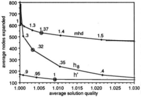
We compare heuristics using performance graphs: A perfonnance graph for h is a plot showing the average in cost (nodes expanded) versus solution quality (C/C·) when A ·( zh) is used and z is varied. See Figure S.l(a). One heuristic is more effective than another in a solution quality region if its performance graph lies below that of the other in that region. For example, in Figure 5.1(a), mhd is more effective than h8 when solution quality better than 1.001 is desired. h' is always more effective than hs and mhd.
2 Model description
Suppose we are given features H1, ... ,Hq. We describe our model for building a heuristic 4 . For simplicity, suppose q=2. Assume:
- (i) R(x,y) is a random variable whenever there exist nodes n,t e G such that x = H1(n,t) andy= H2(n,t).
- (ii) Each R(x,y) has mean JJ[R(x,y)]. There are real numbers {3j such that for all x,y we have
- (iii) R(x,y)=b0+fJ1x+fJ2y+E(x,y), where E(x,y) is a random error. The E(x,y) are independent and normally distributed with mean zero and variance cr2. cr2 is independent of x,y.
- (i), (ii), (iii) describe our statistical model of a heuristic or, simply, heuristic model. Note that they imply that the R(x,y) are independent and normally distributed with common variance u2 · Our model for a single observation is a triplet of numbers (w,x,y) such that
where there exist n, teG satisfying x = H1(n,t), y = H2(n,t), w = k(n,t); E is a value of the random error E(x,y) and w is in the range of R(x,y). We obtain a (finite) set · of such observations, called a sample set. In (2.2) x,y are called independent variables and w is the dependent variable. J.J[R(x,y)] is then estimated by the equation
- m[R(x,y)] = b0 + b1x + b2Y,
which is called a fitted regression line. The parameters /3i of the model (in (2.1)) are estimated as bi, as follows: Let E= ((w1,x1,y1), ... ,(wN,xN,yN)} denote the sample set. Using the method of least squares, the bi'5 are chosen so as to make
4 Our description is along the lines of [Walpole et al., 1989; pp. 357 -62] 0
as small as possible; that is, we minimize the sum-of square-error between the fitted regression line and the observed values of the dependent variable.
Rewriting (2.3) in tenns of the featur~s H1, H2 gives,
m[R(H1,H2)] is called a heuristic fitted to the model (i), (ii), (iii), or, briefly, a fitted heuristic. We say that m[R(H1,H2)l has been obtained from the features H 1, H2 using linear regression and the sample set E.
The situation may be interpreted as follows. Let x 0 = H1(n()ft), Yo= H2(n 0 ,t) be the value of H1,H2 with respect to n 0 and t. The range ofR ( x 0 ,y 0 ) is the set of true distances which occur whenever a pair of nodes have feature values Xo, Yo· p[R(x0 ,y0 )] is the mean value of these distances. Whenever the fitted heuristic is evaluated on a pair of nodes with feature values x 0 , y 0 , it returns an estimate of this mean. The estimate approximates (2.1) with (2.3).
By considering all subsets of a set of features one obtains many heuristic models. For example, seven heuristic models are obtainable from H1, H2, H3 . Two of them yeld the heuristics m[R(H2,H3)] and m[R(H1,H2,H3)].
3 Learning of accurate heuristics: techniques
An accurate heuristic can be built from a small training set T and used to solve any problem of a set P. We call this technique early learning. Continuous learning, on the other hand, is designed for solving small sets of harder problems. In this case learning occurs while solving the problems in the set. The use of either of these methods assumes that perfection in solution quality may, to some extent, be traded for lower use of computing resources.
In both types of learning the initial list of features, is extended by adding to it transformations (square, square roots, etc.) and cross products of its entries. Obvious variations of a feature may also be added. We have found that extending the list of features enables more effective · heuristic models to be built. A systematic study of the best way to extend the list has not been made.
3.1 Early learning of accurate heuristics
We are given a set Hl····,Hq of features and a problem set P. A sample set E is needed for the linear regression. To this end, a small random training set Tis generated. Assume we are given an admissible heuristic h 11 and that h 11 is consistent, or that Mero's [1984] adjustment of A · is used; thus, whenever A · selects a node for expansion, the path to that node from s is optimal [Nilsson, 1980; 2.4.5]. The problems ofT are solved by A ·(h11), and observations are placed in E. In detail, the data collection is as follows: Let cb be a predetermined positive integer, called a control bound. For each problem in T and for each distance w between nodes of G, no more than cb observations (w, x1, ... ,xq) are made. Suppose A ·(h11) is solving a problem in T and that n has just been selected from Open. Let s = n 0 , n1t-.. ,nj+l = n be the path from s ton. Execute if cb observations with w=di have not been collected, add to Ethe observation (di,H1(n,nj), ... ,Hq<n,ni))·
For each problem of T (3.1) is performed once for each node selected from Open.
Input to the statistical routines consists of E and the features H1, ··· ,Hq. Output is a listing of all possible heuristic models with related statistical parameters. This listing is in a convenient order so that the best model can be quickly identified. (See Appendix (1).) We say that the corresponding fitted heuristic, which may now be calculated using linear regression, has been early learned for accuracy. It is applied to the problems of P.
3.2 Continuous learning of accurate heuristics
As before we are given a set H1, .. . ,Hq of features and a problem set P. In continuous learning there is no training set. · Instead, information gained while solving, and partially solving, problems is used to strengthen heuristic knowledge which is then further applied to solving problems in P. This technique is powerful enough to solve problems for which conventional techniques would require too many resources.
3.2.1 Continuous learning: Multiple problem case
We are given an admissible heuristic h4 , which we may assume is consistent. (h 4 could be zero.) Our procedure alternates between two phases. In phase (i) A · is run on each problem of P, but allowed to expand no more than UB nodes per problem, even though no solution may be found. UB is an upperbound determined by space/time considerations of the problem-solving environment. For example, we set UB to 10,000 in the 15-puzzle experiments of Section 6 to run on VAXll/785. In phase (ii) a new heuristic is built using linear regression. The main loop is done ENOUGH times, where ENOUGH, like UB, is determined by the problem-solving environment. For the 15-puzzle we set it to 10. The detailed procedure is:
(3.2) A. h <- h 4
- Do ENOUGH times or until P is empty
- (i) (Solve and make sample set) For each problem in P apply A ·(h) but allow no more than U B nodes to be expanded. If the problem is solved, then remove it from P. During the session use (3.1) to collect the sample set.
- (ii) (Linear regression) If P is empty, then exit. Otherwise consider all possible combinations of the Hi and choose the best heuristic model. (See Appendix: (1)). Let h be the fitted heuristic associated with this model.
C. If Pis not empty then do one of
- (i) (Multiply) Use one of the heuristics built in B(ii) and a multiplier to solve the remaining problems of P.
- (ii) (Single problem accuracy learning) Apply single problem accuracy learning to each problem of P (Section 3.2.2).
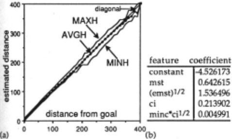
In step C the remaining problems of P may be solved using A ·( zh) where z > 1 and h is one of the heuristics created in B. One may explore for a small z which finds a solution, while expanding no more than UB nodes. Small z's are usually associated with better solution quality than large z's [Bramanti-Gregor et al., 1992). Each iteration of B produces a new heuristic h. One may assess how good h is in two ways: (a) Use model data: See if the confidence interval associated with mean h·-values, at its largest point, is small. Smallness indicates clustering of h near h·. b) Use performance data: Examine the data produced by A ·(h) relative to two properties, (1) A deep search tree is desirable. (2) that the maximum and minimum values of h lie near its average value is also desirable. Such data are easily tabulated and may be plotted (eg., Figure 6.2)
We have observed that a heuristic from B(ii) is not necessarily better than that of the previous iteration. But over several iterations we observe it getting better. The process appears robust in the following sense: if a heuristic causes a shallow tree to be built, the fitted heuristic of the next iteration tends to be accurate, causing a deep tree to be built. There is necessarily a limit to how long one may keep producing more effective heuristics, because the available features contain a finite amount of information.
3.2.2 Continuous learning: Single problem case
The situation is the same as in 3.2.1 except that now P consists of a single difficult problem. The fitted heuristics built in (3.2)8 are now fine-tuned for this one problem. If a solution is not found in B, then C(i) is applied.
In many problems the goal is known in advance. This is true, for example, in sliding tile problems. In this case an adjustment to (3.2) is possible, which fine-tunes the heuristic even more. Recall (cj., (3.1)) that the sample set (~ built in B(i) is based on observations many of which are relatively close to the search tree root . In alternate iterations of (3.2)8, we interchange the role of start and goal. The effect is that, when a fitted heuristic is used, A · is always seeking a goal for which its heuristic has been especially sensitized. In 15-puzzle experiments we find that this improves the performance of (3.2) significantly.
4. Model implications for solution error
Let C denote the solution length returned by A·, and c· denote the optimum solution length. The heuristic model of Section 2 enables probabilistic upper bounds to be placed on solution error, C - c·. Suppose that for each level of certainty we would like to have a bound on expected error, or worst case error, associated with A · solutions. Theorem 4.1, below, provides such bounds. It is proven in [Bramanti-Gregor, 1993). For notational simplicity, we assume two features.
For a given heuristic h we define hy=max(O,h), called a truncated heuristic. Notice that I h1 h·l ~ I h-h·l so hy is at least as accurate as h. Truncated heuristics are used in the experiments of Section 5.
Theorem 4.1 (Upper bound for solution error). Let h = m[R(h1)12)} be a fitted heuristic and suppose A* uses hy. Let x=h1(n), y=h2(n) denote feature values. Let STDP(x,y), STDI(x,y) denote standard errors of mean predicted value and individual prediction, respectively (see Appendix (2)). Then, given 0 <a< 0.5, the probability is at least 1-athat
(4.1) E(c-c·) s sup(taSTDP(h1(n),h2(n)): nt=G}. Also, for any particular problem solved by A·(hT), the probability is at least 1-a that
(4.2) c-e· S sup(taSTDI(h1(n),h2(n)): nt:G}.
t denotes the t-distribution (with I El-3 degrees of freedom). We define the right sides of (4.1), (4.2) to be 100(1-a) % certainty bounds for expected and worst case error, respectively. In our experiments, we have estimated these bounds from the sample set: the supremums of STDP and STDI over G are taken to be the maximum observed values in E. Estimated certainty bounds may be smaller than certainty bounds However, the values we obtain for them in our experiments appear reasonable. See Table 5.3.
5 Experiments on early learning
Early learning was conducted in the 8-puzzle and TSP domains. Fitted heuristics perform 30 to 70% better than the best standard heuristics. Methods for improving a single feature are tested: multiplication and non-linear transformation. The theory's ability to predict solution error is validated by the experimental results.
5.1 8-puzzle experiments
For 8-puzzle experiments we chose features shown in Table 5.1: top and mhd are well-known, and mhd2b has been used in combination with rev for 15-puzzle experiments. For the 8-puzzle, the most effective combination of mhd2b and rev is called h8 in Figure 5.1(a). The set P contains 200 random problems.
| top(n) | tiles-out-of-place Manhattan distance: Ljpj(n) pj(n) is vertical plus horizontal distance of tile i from its goal position. |
| mhd(n) | |
| mhd2(n) | Ljpj(n)2. A variant of mhd |
| blankd(n) | Itbi(n)2. where bj(n) is vertical plus horizontal distance of tile i from empty space. |
| mhd2b(n) rev(n) | l:.i]Jj{n)2bj(n)112 reversal count: Number of tile pairs in correct row or column but in wron order. |
The early learning techniques of Section 3, when applied to the features of Table 5.1 determined the fitted heuristic, h', of Figure 5.1(b). The sample set was obtained by running A ·(mhd) on a training set of size 20 with a control bound of 1. The performance of h' is compared with what we have found to be the best traditional heuristics in Figure 5.1(a). It is substantially better. For example, when solution quality better than 1.01 is desired, it expands 50 to 70% fewer nodes than does its nearest competitor.
5.2 TSP experiments
Experiments on early learning of accurate heuristics were performed on Euclidean TSP's, each built by placing 15
cities randomly on a 100x100 grid. Problem set size was 100. The features of Table 5.2 were used.
| feature | coefficient | |
|---|---|---|
| constant | -3.326942 | |
| top | 0.994649 | |
| top•rev | 0.994649 | |
| mhd | -1.438279 | |
| Figure 5.1(b) Terms of fitted | mhd•rev | -0.321461 |
| heuristic h' built from features | mhd2b | 0.182459 |
| in Table 5.1. First row shows | (mhd2)112 | 3.819975 |
| the constant term. | mhd2 | 0.127242 |
| mi nc | min-cost: maxll:.xminye(x,y),r.ymin,.e(x,y)] where x,y run through all cities which must be exited, entered (respectively) by any path from ctod in V; |
| mst | minimum spanning tree: cost of minimum spanning tree in VU{c} plus min[e(v,d): v e V]; |
| emst | enhanced mst: cost of a depth first traversal of minimum spanning tree plus min[e(v,d): v e V];. |
| nnbr | nearest neighbor: connect c to d by a path that always goes to the nearest unvisited city. |
| ci | cheapest insertion: Build a path from c to d by selecting the next city randomly and inserting it into the partial path at that point which minimizes the increase in ath len th. |
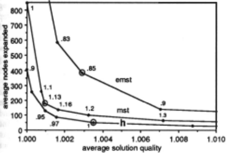
The sample for linear regression was generated by A·(mst) on 20 random training problems using a control bound of 1. The fitted heuristic obtained is shown in Figure 5.2(b) and in Figure 5.2(a) its performance is compared with that of the two strongest features of Table 5.2. The fitted heuristic performs substantially better. For example, when solution quality better than 1.01 is desired, it expands from 30 to 50% fewer nodes than the nearest competitor (mst).
| --~re-a_t_u-re _____ | c_o_e~f~fi-ci~e-n_t_ |
|---|---|
| constant mst nnbr minc•(emst)l/2 minc•(nnbr)l/2 minc 00 (ci)l/2 | -1.829112 0.549157 0.596828 0.014057 -0.037609 0.011786 |
5.3 Building models from a single feature
Suppose we are given a single feature. The fitted heuristic associated with a one-feature model has the form v 0 + z 0 h. z 0 is the optimal multiplier for h from a least-square-error point of view. Its location on performance graphs for several heuristics is shown by an open circle in figures S.l(a), 5.2(a) and 5.3. The optimal multiplier may be interpreted as follows: Decreasing z towards z 0 improves solution quality with a small penalty in node expansion; further decreases in z, below z 0 , cause small improvements in solution quality, at higher penalty in node expansion.
Sometimes a single feature contains more useful information than is revealed by using it alone. For example, consider h8 of Figure 5.1(a) as if it were a feature, a kind of "black box". We use early learning to select the best heuristic model for the features {h8i/4: 1 SiS 8}.
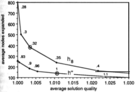
The resulting fitted heuristic is a linear combination of three terms: h8 1 1 4 , hi1 4 , hi. Its performance is compared to that of h8 in Figure 5.3. It is substantially better. To us this indicates that, once a good feature is known, the optimal way to exploit the information it contains may not be intuitive; and linear regression is a powerful tool for accessing this information.
5.4 Model-predicted bounds on solution error
We applied Theorem 4.1 to the fitted heuristics discussed above to see if the certainty bounds on solution error predi cted by the model appear consistent with observed values. Table 5.3 shows that they are. The bottom two entries in parts (a) and (b) of the table refer to z(mst) and z(emst) respectively, where the multiplier z is chosen "optimally" in the sense of Section 5.3.
| certainty | observed average | ||
|---|---|---|---|
| fitted heuristic | 95% | 84% | value of error |
| Figure 5.1(h') | 0.87 | 053 | 0.18 |
| Figure 5.3(h") | 0.97 | 059 | 0.21 |
| Figure 5.2(h) | 2.30 | 1.40 | 121 |
| optimal mst | 1.81 | 1.10 | 027 |
| optimal emst | 327 | 1.99 | 1.00 |
(a) Estimated certainty bounds for expected error
| b d do/. b certamty oun an o o servatlons b 1 eow | ||||||
|---|---|---|---|---|---|---|
| 99.9% | 95% | 84% | ||||
| fitted heuristic | bound | % | bound | % | bound | % |
| Figure 5.1 (h') | 5.48 | 100 | 2.99 | 99 | 1.82 | 91 |
| Figure 5.3(h") | 5.63 | 100 | 3.08 | 100 | 1.87 | 89 |
| Figure 5.2(h) | 19.47 | 100 | 10.64 | 98 | 6.47 | 95 |
| optimal mst | 38.71 | 100 | 21.15 | 100 | 12.86 | 100 |
| optimal emst | 55.26 | 100 | 30.20 | 100 | 18.36 | 100 |
(b) Estimated certamty bounds for worst case error
Table 5.3. Estimated certainty bounds vs. observed values.
6 Experiments on continuous learning
Experiments on continuous learning were performed in the 15-puzzle and the TSP with 20 cities. These domains are apftealing because their problems typically contain over 10 5 paths to goal, providing a combinatorially explosive environment on which to test the effectiveness of the continuous learning method. In such an environment A · cannot be used when high quality solutions are required, unless it is given a powerful heuristic to guide the search.
It is relevant to know the cost in time of learning since learning occurs as a problem is solved. The learning involves: (1) Sampling; on average our sample sets contain 700 observations with 7 variables (features) to be evaluated. (2) Model selection; a statistical package determines the best models. (3) Linear regression to determine the coefficients for the selected model. In our experiments, approximately 2.5% of the total time used to solve a problem is spent in collecting the sample; the other two activities add only a negligible amount, 0.1% on average.
6 .1 IS-puzzle experiments
Our problem sets are subsets of a random set of 1 00
problems which have been solved optimally by IDA · and are listed in Korf [1985). We use these problems because their optimal solution length is known, helping us evaluate our technique. Unlike the IDA · experiments, we are not seeking optimal solutions. We are interested in high quality solutions at low time-complexity; but, more importantly, we are exploring the extent to which our techniques enable accurate high-performance heuristics to be built in a combinatorially explosive environment.
The three experiments described below indicate that this can be done. Although these experiments are on problems of different difficulty levels and use different techniques, there is an overall pattern:
- (i) solution quality, on average, is within 2% of optimal.
- (ii) we generate on average 165,774 nodes (as opposed to 361,907,110 for optimal IDA · solutions on the same set of problems) and have on average 8 linear regression sessions per problem; during each of these sessions a new heuristic is "learned, or built, from previous experience".
(iii) the final heuristic, in the sequence of fitted heuristics that are built, is so accurate that it enables A · to solve the problem within a few moves of optimal, often optimally, while generating less than 20,000 nodes. See Figure 6.1.
We performed two experiments in multiple problem learning and one in single problem learning. Table 6.1 summarizes the results. Optimal solution length, c·, ranges from 41 to 66 in Korfs sample set. We take it as a rough indication of problem difficulty. Experiments 1, 2 perform multiple problem learning on the easiest and second easiest 10 problems of the sample. The algorithm is (3.2) of Section 3.2.1. It sometimes performs single problem learning (step C(ii)), and this happened in five of the 20 problems we considered. The "hardest" of Korfs problems are the nine ones with C* ~60. We arbitrarily picked five of these for single problem learning in Experiment 3.
| feature | coefficient |
|---|---|
| constant mhd (mhd)2 mhd2 rev blankd | -0.085928 0.747448 -0.670539 0.262524 1.691776 0.012312 |
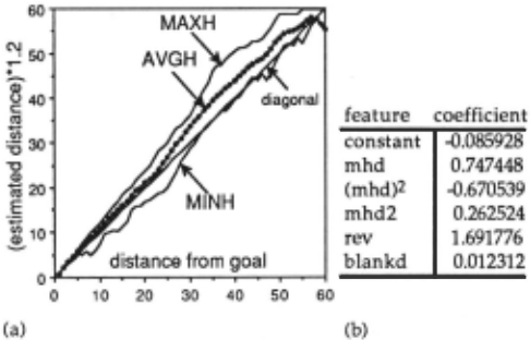
We used the features of Table 5.1 plus the additional feature h8 of Figure 5.1(a). (3.2) was implemented as follows: UB=10,000 and ENOUGH = 10; that is, in each problem no more than 10,000 nodes are expanded and the main loop is performed at most 10 times. If a problem is not solved at this point, then another iteration is allowed with multiplier 1.2 (Step C(i)). Any problem still remaining unsolved is now subjected to single problem learning (Step C(ii)). In the latter, we were prepared to have a 12th iteration with multiplier 1.4, if necessary, but this was never required. In all experiments the heuristic used in the first iteration (ie., ha in (3.2)) is mhd. The control bound during learning was set so as to give up to 20 readings for each distance from goal.
To give a feel of the heuristics built during the experiments, Figure 6.1 describes the heuristic produced in the 10th iteration of the first problem in Experiment 3 and the behavior of the multiplied version that solved the problem As can be seen, the multiplied version never deviates by more than 9 from true values. In our judgement, this is remarkably accurate.
| nodes generated | ||||||
|---|---|---|---|---|---|---|
| KorfNo. | c• | c;c• | z | A• | IDA• | |
| 55 | 41 | 1.00 | 1.0 | 32,246 (2) | 927,212 | |
| 16 | 42 | 1.00 | 1.0 | 296,534 (15) | 17,984,051 | |
| 42 | 42 | 1.00 | 1.0 | 28,444 (2) | 877,823 | |
| 79 | 42 | 1.00 | 1.0 | 52,574 (3) | 540,860 | |
| 71 | 44 | 1.00 | 1.0 | 96,240 (5) | 8,885,972 | |
| 85 | 44 | 1.00 | 1.0 | 51,004 (3) | 2,725,456 | |
| 97 | 44 | 1.00 | 1.0 | 69,654 (4) | 1,002,927 | |
| 12 | 45 | 1.00 | 1.0 | 28,464 (2) | 546,344 | |
| 61 | 45 | 1.00 | 1.0 | 79,056 (4) | 7,096,850 | |
| 86 | 45 | 1.00 | 1.0 | 51,048 (3) | 2,304,426 | |
| Experiment 1 | 1.00 | 1.0 | 78,426 (4.3) | 4,285,191 | ||
| 9 | 46 | 1.00 | 1.0 | 53,668 (3) | 1,1650696 | |
| 13 | 46 | 1.09 | 1.0 | 408,306 (21) | 11,861,705 | |
| 19 | 46 | 1.00 | 1.0 | 54,992 (3) | 1,280,495 | |
| 93 | 46 | 1.09 | 1.2 | 208,828 (11) | 1,599,909 | |
| 30 | 47 | 1.00 | 1.2 | 207,964 (11) | 2,196,593 | |
| 47 | 47 | 1.00 | 1.0 | 45,956 (3) | 1,411,294 | |
| 65 | 47 | 1.00 | 1.2 | 431,000 (22) | 18,997,681 | |
| 75 | 48 | 1.00 | 1.2 | 430,100 (22) | 42,772,589 | |
| 23 | 49 | 1.00 | 1.0 | 375,536 (19) | 15,971,319 | |
| 39 | 49 | 1.04 | 11 | 214,252 (11) | 19,355,806 | |
| Experiment | 2 | 1.0022 | 1.1 | 243,058(12.3) | 11,709,809 | |
| 33 | 60 | 1.00 | 12 | 210,456 (11) | 480,637,867 | |
| 66 | 61 | 1.00 | 12 | 217,016 (11) | 1,957,191,378 | |
| 15 | 62 | 1.03 | 1.0 | 82,650 (5) | 543,598,0673 | |
| 43 | 64 | 1.03 | 11 | 215,122 (11) | 41,124,767 | |
| 88 | 65 | 1.03 | 1.2 | 204,278 (11) | 6,009,130,748 | |
| Experiment 3 | 1.018 | 1.16 | 185,908(9.8) | 1,806,336,565 | ||
6.2 TSP experiments
Our TSP experiments are on maps of 20 cities and the problem set consists of 20 randomly generated problems. The optimal solution for each problem is obtained by running A·(mst) on the Cray Y-MP8/864 of the Ohio Supercomputer Center, due to the large space require ments for some of the problems. The optimal solutions are used to evaluate the effectiveness of continuous learning. In addition, the number of nodes generated by A ·(mst) provide a basis for evaluating the corresponding cost when a fitted heuristic is used.
The experiments reveal the following:
- (i) All problems are solved optimally.
(ii) On average 9,768nodes are generated per problem as opposed to 32,282 with A·(mst).
(iii) All problems are solved within three linear regression sessions. Each session produces a new fitted heuristic. The final heuristic is so accurate that enables A · to solve the problems optimally, while generating less than 10,000 nodes, even on problems for which A ·(mst) generates more than 100,000 nodes.
We performed two experiments in multiple problem learning, each with 10 problems. The algorithm is (3.2) of Section 3.2.1, where UB is set so as to limit nodes generated to 10,000 and ENOUGH to 10. The control bound, cb, is set so as to give up to 20 readings for each path interval of length 10. Step C is never executed because all problems are solved in step B.
Figure 6.2 describes the heuristic of Experiment 1 which solves six problems at the second iteration (b) and shows its behavior during problem solving (a). It is very accurate: all values lie close to the diagonal.
7. Conclusions
Our regression model (Section 2) has several properties which are only approximately true in the application. One is the normality assumption (iii), especially that the variance a2 is constant. Another occurs in "continuous learning" (sections 3, 7) because our observations do not always have correct values for the dependent variable in that context. Nevertheless, our experimental results reveal high quality A· performance. The heuristics of figures 6.1, 6.2 are typical of what we observed: apparent "bounded" error, a rare phenomenon among heuristics. Furthermore, the statistical measurements regarding validity of the chosen regression models (Appendix(})) are positive.
We believe that the techniques we describe have generality: A small number of basic problem insights, represented here as features (eg., Tables 5.1, 5.2), when properly combined yield very effective heuristic functions.
However, the appropriate combination is non-intuitive (eg., figures 5.1(b), 5.2(b), 6.1(a), 6.2(b). Statistical methodology provides an excellent tool.
Appendix
(1) Criterion for selecting a heuristic model: In selecting one linear regression model over another we were able to insist that F-tests and t-tests be 0.0001. Almost always the adjusted-R 2 was 2 0.90, often 2 0.95. After looking for a small root mean square error and standard error in parameter estimate, we favor models that use a small number of features. The selection process is automatable
(2) Standard error of mean predicted value and of individual prediction (See Theorem 4.1): This terminology is from the SAS statistical system for data analysis. We relate it to other concepts: STDP(x 0 ,y 0 )=s[C(x 0 y 0 )]11 2 , where sis root mean square error, C(x 0 yoJ=(x 0 ,y 0 )(X·X)-l(x 0 ,y 0 ), X is a matrix containing values of the independent variables from the sample, and · denotes transpose. Similarly, STDI(x 0 ,y 0 )=s[1+C(x 0 ,y 0 )Jll2. See (Walpole et al., 1989; Sections 9.5, 10.5).
@inproceedings{ijcai1993p149,
  title     = {The Statistical Learning of Accurate Heuristics},
  author    = {Bramanti-Gregor, Anna and Davis, Henry W.},
  booktitle = {Proceedings of the Thirteenth International Joint Conference on
               Artificial Intelligence, {IJCAI-93}},
  publisher = {International Joint Conferences on Artificial Intelligence},
  editor    = {Ruzena Bajcsy},
  pages     = {1079--1086},
  year      = {1993},
  note      = {Machine Learning},
  url       = {https://ijcai.org/proceedings/1993/149},
}
TY - CPAPER TI - The Statistical Learning of Accurate Heuristics AU - Bramanti-Gregor, Anna AU - Davis, Henry W. T2 - Proceedings of the Thirteenth International Joint Conference on Artificial Intelligence, IJCAI-93 PB - International Joint Conferences on Artificial Intelligence PY - 1993 SP - 1079 EP - 1086 UR - https://ijcai.org/proceedings/1993/149 ER -Copied
Machine-readable versions of this paper, for tools and AI agents:





