
Rule-Based Regression
Proceedings of the Thirteenth International Joint Conference on Artificial Intelligence. Machine Learning. Pages 1072-1077.
© 1993 International Joint Conferences on Artificial Intelligence
Abstract
While decision trees have been used primarily for classification, they can also model regression or function approximation. Like classification trees, regression trees often yield excellent results with the advantages of strong explanatory capabilities and dymunic feature selection in high dimensions. In this paper, we contrast techniques for inducing classification and regression trees. We then present an altemative model of regression rules. A new technique for inducing decision rules for regression is described. This model of ordered disjunctive normal form rules, is potentially stronger and more compact than decision trees. Preliminary experimental results suggest that the new procedure is effective and can often exceed regression tree performance.
- [Anderberg, 1973] Anderberg, M. Cluster Analysis for Applications. New York: Academic, 1973.
- [Apte, Weiss, and Grout, 1992] Apte, C., Weiss, S., and Grout, G. "Predicting Defects in Disk Drive Manufacturing: A Case Study in High-Dimensional Classification." In Proceedings of IEEE CAIA -93, 1993,212-218.
- [Breiman, Friedman, Olshen, and Stone, 1984] Breiman, L., Friedman, J., Olshen, R., and Stone, C. Classification and Regression Tress. Monterrey, Ca.: Wadsworth, 1984. [Clark and Niblett, 1989]
- Clark, P. and Niblett, T. "The CN2 Induction Algorithm." Machine Learning. 3 (1989) 261-283.
- [Craven and Wahba, 1979] Craven, P. and Wahba, G. "Smoothing Noisy Data with Spline Functions. Estimating the Correct Degree of Smoothing by the Method of Generalized Cross-Validation." Numer. Math. 31 (1979) 317-403.
- [Detrano et al ., 1989] Detrano, R., Janosi, A., Steinbrunn, W., Pfisterer, M., Schmid, J., Sandhu, S., Guppy, K., Lee, S. and Froelicher, V. "International application of a new probability algorithm for the diagnosis of coronary artery disease." American Journal of Cardiology. 64 (1989) 304-310.
- [Efron, 1988] Efron, B. "Computer-Intensive Methods in Statistical Regression." SIAM Review. 30:3 (1988) 421-449.
- [Fayyad and Irani, 1992] Fayyad, U. and Irani, K. :'The Attribute Selection Problem in Decision Tree Generation." In Proceedings of AAAI-92. San Jose, 1992, 104-110.
- [Fisher, 1936] Fisher, R. "The Use of Multiple Measurements in Taxonomic Problems." Annals of Eugenics. 7 (1936) 179-188.
- [Friedman, 1991] Friedman, J. "Multivariate Adaptive Regression Splines." Annals of Statistics. 19:1 (1991) 1-141.
- [Friedman and Stuetzle, 1981] Friedman, J. and Stuetzle, w. "Projection Pursuit Regression." J. Amer. Stat. Assoc. 76 (1981) 817-823.
- [Girosi and Poggio, 1990] Girosi, F. and Poggio, T. "Networks and the Best Approximation Property." Biological Cybernetics. 63 (1990) 169-176.
- [Hastie and Tibshirani, 1990] Hastie, T. and TibshinUli, R. Generalized Additive Models. Chapman and Hall, 1990. [Lebowitz, 1985]
- Lebowitz, M. "Categorizing Numeric Information for Generalization." Cognitive Science. 9 (1985) 285-308.
- [Lin and Kernighan, 1973] Lin, S. and Kernighru1, B. "An Efficient Heuristic for the Traveling Salesmru1 Problem." Operations Research. 21:2 (1973) 498-516.
- [McClelland and Rumelhart, 1988] McClelland, J. and Rumelhart, D. Explorations in Parallel Distributed Processing. Cambridge, Ma.: MIT Press, 1988.
- [Michalski, Mozetic, Hong, and Lavrac, 1986] Michalski, R., Mozetic, I., Hong, J., and Lavrac, N. "The Multi-purpose Incremental Learning System AQ15 and its Testing Application to Three Medical Domains." In Proceedings of AAAI-86. Philadelphia, Pa., 1986, 1041-1045.
- [Quinlan, 1986] Quinlan, J. "Induction of Decis;t>n Trees." Machine Learning. 1 (1986) 81-106.
- [Quinlan, 1987] Quinlan, J. "Simplifying Decision Trees." International Journal of Man-Machine Studies. 27 (1987) 221-234.
- [Ripley, 1993] Ripley, B. "Statistical Aspects of Neural Networks." In Proceedings of Seminair Europeen de Statistique. Chapmru1 and Hall, London, 1993, in press.
- [Scbeffe, 1959] Scbeffe, H. The Analysis of Variance. New York: Wiley, 1959.
- [Weiss and Indurkhya, 1991] Weiss, S. and Indurkhya, N. "Reduced Complexity Rule Induction." In Proceedings of /JCA/-91. Sydney, 1991, 678-684. IJCAI
- [Weiss and Kapouleas, 1989] Weiss, S. and Kapouleas, I. "An Empirical Comparison of Pattern Re:::ognition, Neural Nets, and Machine Learning Classification Methods." In Proceedings of /JCAJ-89. Detroit. Michigan, 1989, 781-787.
- [Weiss ru1d Kulikowski, 1991] Weiss, S. ru1d Kulikowski,
References were extracted automatically from the PDF and may contain errors.
Full text extracted automatically from the PDF; figures, tables and equations may differ. The PDF is the version of record.
1 Introduction
Regression or function approximation is a principal task of statistical analysis. Given samples of output (response) variable y and input (predictor) variables { x 1 ... x 0 }, the task is to find a mapping y = f({x 1 ... x 0 }). Relative to the space of possibilities, finite samples are far from complete, and a pre-defined model is needed to concisely map { x 1 ... x 0 } toy. Accuracy of prediction, i.e. generalization to new cases, is of primary concem. Regression differs from classification in that the output variable y can be continuous, whereas in classification y is strictly categorical. From this perspective, classification can be thought of as a subcategory of regression.
The classical statistical model is linear least-squares regression [Scheffe, 1959]. Developed and refmed over many years, linear regression has proven quite effective for many real-world applications. Clearly the elegant and computationally simple linear model has its limits, and more complex models may fit the datc'l better. With the increasing computational power of computers and with larger volumes of data, interest has grown in pursuing altemative nonlinear regression methods. Nonlinear regression models have been explored by the statistics research community and many new effective methods have emerged [Efron, 1988] including projection pursuit [Friedman and Stuetzle, 1981] <md MARS [Friedman, 1991]. Methods for nonlinear regression have been developed outside the mainstream statistics research community. Neural networks trained by back-propagation [McClelland and Rumelhart, 1988] are another model for nonlinear regression. Altemative models are also found in numerical analysis [Girosi and Poggio, 1990]. Au overview of many different regression models, with application to classification, is given in [Ripley, 1993].
As a pure problem type, classification is more conunonly encountered than regression. Still regression methods c<m be used to solve classification problems, for example neural networks are often applied to classification problems. Within the machine leamiug research cOimnunity, classification methods have been emphasized. Recursive partitioning methods, such as ID3 decision tree induction [Quinlan, 1986], have been applied exclusively to classification tasks. Less widely known is that decision trees are also effective in regression. The CART program, developed in the statistical research community, induces both classification and regression trees [Breiman, Friedman, Olshen, and Stone, 1984]. These regression trees are strictly binary trees, a representation which naturally follows from intensive modeling using continuous variables. 1
In terms of performance, regression trees often are competitive in perfonnance to other regression methods [Breiman, Friedman, Olshen, and Stone, 1984] . Regression trees are noted to be particularly strong when there are many higher order dependencies among the input variables [Friedman, 1991]. The advantages of the regression tree model are similar to classification trees. Two principal advantages can be cited: (a) dynamic feature selection and (b) explanatory capabilities. Tree induction methods are extremely effective in fmding the key attributes in high dimensional applications. In most applications, these key features are only a small subset of the original feature set. A characteristic of decision trees that is often cited is its capability for explanation in terms acceptable to people. It helps answer Why was this decision made? On the negative side, decision trees cannot represent compactly many simple functions, for example linear functions. A second weakness is that the regression tree model is discrete, yet predicts a continuous variable. For function approximation, the expectation is a smooth continuous function, but a decision tree provides discrete regions that are discontinuous at the boundaries. All in all though, regression trees often produce strong results, and for many applications their advantages strongly outweigh their potential disadvantages.
1 A. ~mparative study by [Fayyad and Irani ,_ I ?92) suggests that binary cl~sification trees are somewhat more predictive even for categorical variables.
Both decision trees and decision rules can be described as disjunctive normal fonn (DNF) models. Decision rules are similar in characteristics to decision trees, but they also have some potential advantages: (a) a stronger model (b) often better explanatory capabilities. Unlike trees, DNF rules need not be mutually exclusive. Thus, their solution space includes all tree solutions. These rules are potentially more compact ~md predictive than trees. Decision rules may also offer greater explanatory capabilities than trees because as a tree grows in size, its explanatory capability diminishes. In this paper we describe a new method for inducing regression rules. The method takes advantage of the close relationship between classification and regression and provides a unifonn ~md general model for dealing with both problems. Empirical results suggest that the method is effective and cru1 induce solutions that are often superior to decision trees.
2 Methods
2.1 Measuring Performance
The objective of regression is to mmumze the disumce between the srunple output values, Yi ~md the predicted values y' i" Two measures of distru1ce are cmmnonly used. The classical regression measure is equation 1, the average squared distance between yi and y' i' i.e. the variance. It leads to ru1 elegant fonnulation for the linear least squares model. The mean absolute disumce (deviation) of equation 2 is used in least absolute deviation regression, and is perhaps the more intuitive measure. In keeping with the spirit of methods having strong explanatory capabilities, we will measure perfonnance by mean absolute disumce. This is a measure of the average error of prediction for each Yi·
The regression problem is sometimes described as a signal and noise problem. The model is extended to include a stochastic component c: in equation 3. Thus, the true function may not produce a zero error distru1ce. In contrast to classification where the labels are assumed correct, for regression the predicted y values could be explained by a number of factors including a random noise component, c:, in the signal, y.
Because prediction and generalization are the primary concem, estimates based on training cases alone are inadequate. The principles of predicting perfonn~mce on new cases are analogous to classification, but here the meru1 absolute distru1ce is used as the error rate, Err. The best estimate of true perfonmmce of a model is the error rate on a large set of independent test cases. When large samples of data are unavailable, the process of train and test is simulated, preferably by rru1dom resmnpling. In our experiments, we used cross-validation to estimate predictive perfonnru1ce.
2.2 Regression by Tree Induction
In this section, we contrast regression tree induction with classification tree induction. Like classification trees, regression trees are induced by recursive partitioning. The solution takes the fonn of equation 4, where Ri are disjoint regions, and ki are consumt values.
Regression trees have the srune represenuttion as classification trees except for the tenninal nodes. The decision at the tenninalnodes is to assign a case a consumt y value. This value is detennined by the meru1 (or mediru1) of the training cases falling into that tenninal node. 2 Figure 1 is an example of a binary regression tree. All cases reaching shaded tenninal node 1 (xI ~ 3) are assigned a constant value of y=lO.
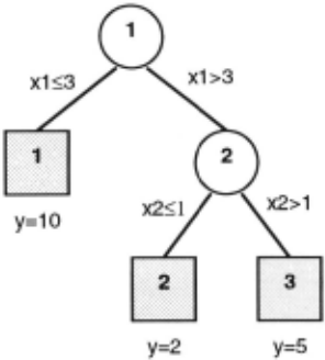
Tree induction methods usually proceed by (a) finding a covering set for the training cases ru1d (b) pruning the tree to the best size. Although classification trees have been more widely studied, a similar approach can be applied to regression trees. We assume the reader is fruniliar with classification trees, and we cite only the differences in binary tree induction [Breimru1, Friedmm1, Olshen, ;md Stone, 1984, Quinlan, 1986, Weiss and Kulikowski, 1991]. In many respects, regression tree induction is more straightforward. For classification trees, the error rate is a poor choice for node splitting, and alternative functions such as entropy or gini are employed. For regression tree induction, the minimized function, i.e. absolute distance, is most satisfactory. At each node, the single best split that minimizes the mean disumce is selected. Splitting continues until fewer than k cases are covered by a node, or until all cases within the node have the identical value of y.
The goal is to find the tree that generalizes best to new cases, and this is often not a full covering tree, particularly in presence of noise or weak features. The pruning strategies employed for classification trees are equally valid for regression trees. Like the covering procedures, the only substantial difference is that the error rate is measured in terms of mean absolute distance. One popular method is the weakest-link pruning strategy [Breiman, Friedman, Olshen, <md Stone, 1984]. For weakest-link pruning, a tree is recursively pruned so that the ratio delta/n is minimized, where n is the number of pruned nodes and delta is the increase in error. Weakest link pruning has several desirable characteristics: (a) it prunes by training cases only, so that the remaining test cases are relatively independent (b) it is compatible with resampling.
2 Within a partition, the median is the m.inim.izer of mean absolute distance. In our experiments, the mean and median were quite close in both apparent and predicted errors. The median always had a reduced mean error on the training cases, but the mean was often slightly better in prediction.~ . This may be due to the relatively small sample for each partition.
2.3 Regression by Rule Induction
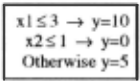
Both tree and rule induction models find solutions in disjunctive normal form, and the model of equation 4 is applicable to both. Each rule in a rule set represents a single partition or region Ri. Unlike the tree regions, the regions for rules need not be disjoint. With non-disjoint regions, several rules may be satisfied for a single sample. Some mech<mism is needed to resolve the conflicts in ki, the constmlt values assigned, when multiple rules, i.e. the Ri regions, are indicated. One standard model (e.g. [Weiss and lndurkhya, 1991]) is to order the rules. The first rule that is satisfied is selected as in equation 5.
Figure 2 is an example of an ordered rule set corresponding to the tree of Figure I. All cases satisfying rule 3, <md not rules I and 2, are assigned a value of y=5.
Given this model of regression rule sets, the problem is to find procedures that effectively induce solutions. Such methods can be described in terms similar to the major components of most tree <md rule induction techniques: (a) find a covering set and (b) prune the rule set to an appropriate size. Improved results can be achieved when an additional technique is considered: (c) refine or optimize a rule set.
2.3.1 A Reformulation of tbe Regression Problem
For rule-based regression, a covering strategy analogous to the classification tree strategy could be specified. A rule could be induced by adding a single component at a time, where each added component is the single best minimizer of dis~'Ulce. As usual the constant value ~ is the mean (or medim1) of the region formed by the current rule. As the rule is extended, fewer cases are covered. When fewer than a minimal number of cases are covered, rule extension terminates. The covered cases are removed and rule induction can continue on the remaining cases. This is also the regression analogue of rule induction procedures for classification [Michalski, Mozetic, Hong, and Lavrac,
1986, Clarlc and Niblett, 1989].
Instead of this approach, we propose an unusual strategy of mapping the regression covering problem into a classification problem. The motivation for this mapping is based on a number of factors, all related to the extra information given in the regression problem: the natural ordering of { yi} by magnitude: if i > j then yi > y ..
Let { Ci} be a set consisting of an arbitrary J number of classes, each class containing approximately equal values of { Yi}. To solve a classification problem, we expect that the classes are different from each other, and that patterns cru1 be found to distinguish these classes. Should we expect classes formed by an ordering of {yi} to be a reasonable classification problem? There are a numbers of reasons why the answer is yes, particularly for a rule induction procedure.
The most obvious situation is the classical linear relationship. In this instance, by defmition, some ordering of {xti···xni} corresponds to the ordering of {yi}. Although classical methods are very strong in compactly determining linear functions, most interest in modem methods centers around their potential for finding nonlinear relationships. For nonlinear functions, we know that there is no such ordering of {xti···Xru} corresponding to the {yi}. Still, we expect that the true function is smooth, and in a local region the ordering relationship will bold. In terms of classification, we know that a class cj with similar values of y is quite different than class ck with much lower values of y. For a nonlinear function within a class of similar values of y, some of these y have very similar values of {x 1 i ... xni}. These correspond to some local region of the function. However, it is also true that some identical values of y can have very different {x 1 i ... xni} so that multiple clusters can be found within the class. Because rule induction methods do not cover a class with a single rule, the expectation is that multiple patterns will be found to cover these clusters.
2.3.2 A Covering Rule Set
With this transformation, rule induction algorithms for classification can be applied. We will consider those induction methods that fully cover a class before moving on to induce rules for the next class. At each step of the covering algorithm, the problem is considered a binary classification problem for the current class C. versus all C. where j > i, i.e. the current class versus Ute remaining classes. When a rule is induced, its corresponding cases are removed and the remaining cases are considered. When a class bas been covered, the next class is considered. An example of such a covering algorithm is found in [Weiss and Indurkhya, 1991]. The covering method is identical for classification and regression. However, one distinction is that the regression classes are transient labels that are replaced with the mean of the y values for the cases covered by each induced rule. Because the rules are ordered and multiple rules may be satisfied, the means are derived only from those instances where the rule is the ftTSt to be satisfied.
The specification of these classes does not use any information beyond the ordering of y. No information about the true nature of the underlying function is known. Within this restricted environment, the goal is to make the y values within one class most similar and y values across classes most dissimilar. We wish to assign the y values to classes such that the overall distance between each yi and its class mean is minimum.
Figure 3 describes an algorithm (P-Class) for assigning the values { Yi} to k classes. Essentially the algorithm does the following: (a) sorts the y values; (b) assigns approximately equal numbers of contiguous sorted Yi to each class; (c) moves a Yi to a contiguous class when that reduces the global distance Err from each Yi to the mean of its assigned class; (d) if no move reduces the overall distance, classes with the same means are combined, and the algorithm halts. The task of transforming a numerical variable into classes is known as numeric categorization. P-Class is a type of statistical clustering method that mmumzes a distance measure [Anderberg, 1973]. Altemative categorization methods that do not depend on distance measures are described in [Lebowitz, 1985].
Input: { y} a set of output values
Initialize n := number of cases , k := number of classes repeat for each Class; Class; := next n/k cases from list of sorted y values end
repeat for each Class; (until no change for any class)
repeat for each case j in Class;
I . Move Case;· to Class;_ 1 , compute Err new if Err new> Err old return Caseij to C; 2. Move Case; . to Classi+l' compute Err new if Err new> Err old return Caseij to C; next Casej in Class; Next Class; repeat for each Class; (until no change for any class) If Mean(Class;) = Mean(Classj) then Combine Class; and Classi end
Figure 3: Composing Pseudo-Classes (P-Class)
Given a fixed number of k classes, this procedure will relatively quickly assign the yi to classes such that the overall distances are minimized. Because the underlying function is unknown, it is not critical to have a global minimum assignment of the Yi· This procedure matches well to our stated goals for ordering the Yi values. The obvious remaining question is bow do we determine k, the number of classes? Unfortunately, there is no direct answer, and some experimentation is necessary. However, as we shall see in Section 3, there is empirical evidence suggesting that results are quite similar within a local neighborhood of values of k. Moreover, relatively large values of k, which entail increased computational complexity for rule induction, are typically necessary only for noise-free functions that can be modeled exactly. Analogous to comparisons of neural nets with increasing numbers of hidden units, the trends for increasing numbers of partitions become evident during experimentation.
One additional variation on the classification theme arises for rule induction schemes that cover one class at a time. The classes must be ordered, and the last class typically becomes a default class to cover situations when no rule for other classes is satisfied. For regression, having one default partition for a class is unlikely to be the best covering solution, and instead the remaining cases for the last class are repeatedly partitioned (by P-Class) into 2 classes until fewer than m cases remain.
An interesting characteristic of this transformation of the regression problem is that we now have a uniform and general model that once again relates both classification and regression. If the Yi values are discrete and categorical, P Class merely restates the standard classification problem. For example, if all values of Yi are either 0 or I, then the result of P-Class will be be 2 classes.
We have described the motivation for expecting reasonable results from this covering procedure. Although this transformation may yield good covering sets, additional procedures are necessary for a complete solution.
2.3.3 Pruning tbe Rule Set
Typical real-world applications have noisy features that are not fully predictive. A covering set, particularly one composed of many continuous variables, will be far too overspecialized to produce the best results. For classification, relatively few classes are specified in advance. For regression, we expect many smaller groups because values of Yi are likely to be quite different.
The result of pruning a covering rule set, RS 0 , is a series of progressively smaller rules sets {RS 0 ··· RSi ... RSn}. The objective is to pick the best one, usually by some form of error estimation. Model complexity and future perfonnance are highly related. Both too complex or too simple a model can yield poor results, the objective being to find just the right size model. Independent test cases or resampling by cross-validation are effective means of estimating future performance. In the absence of these estimates, approximations, such as GCV [Craven and Wahba, 1979, Friedman, 1991], as described in equation 6, have been used in the statistics literature to estimate performance 3 . Both measures of training error and model complexity are used in the estimates. C(M), is a measure of model complexity expressed in terms of parameters estimated or tests performed, where C(M) is assumed to be less than n, the number of cases.
We noted that for trees the usual pruning techniques C<Ul be applied with the substitution of mean absolute distance for the classification error rate. As in weakest-link tree pruning, the same ratio of delta/n can be recursively minimized for weakest-link rule pruning. The intuitive rationale is to remove those parts of a rule set that have the least impact on increasing the error. Pruning rule sets is usually accomplished by either deleting complete rules or single rule components [Quinlan, 1987, Weiss and lndurkhya, 1991]. In general, rule pruning (for both classification and regression) is less natural and far more computationally expensive than tree pruning. Tree pruning has a natural flow from set to subset. Thus a tree can be pruned from bottom up, typically considering the effect of removing a subtree. Non-disjoint rules have no such natural pruning order, for example every component in a rule is a candidate for pruning and may affect all other rules that follow it in the specified rule order.
3 GCV is an acronym for generalized cross-validation. but only the apparent error on training cases is used and not true cross-validation by resampling.
There is a major difference in pruning regression rules vs. classification rules. For classification, deleting a rule or a rule component has no effect on the class labels. For regression, pruning will change the mean-values of y for the regions. Even the deletion of a rule will affect other region meru1s because the rules are ordered and multiple rules may be satisfied. This characteristic of rule pruning for regression adds substantial complexity to the task. However, by assuming that the mean-values of y remain unchru1ged during the evaluation of candidate rules to prune, a pruning procedure can achieve reasonable computational efficiency at the expense of some loss in the accuracy of evaluation. Once the best rule or component for deletion is selected, the means of all regions can then be re-evaluated.
Even for classification rules, rule pruning has some inherent weaknesses. For example, rule deletion will often create a gap in coverage. For classification rules though, it is quite feasible to develop an additional procedure to refme and optimize a rule set. To a large extent, this overcomes the cited weakness in pruned rules sets. A similar refinement and optimization procedure can be developed for regression ru1d is described next.
2.3.4 Rule Refinement and Optimization
Given a rule set RSi, can it be improved? This question applies to any rule set, although we are mostly motivated by trying to improve the pruned rules sets {RS 0 ... RSi ... RSn}. This is a combinatorial optimization problem. Using error measure Err(RS), can we improve RSi without changing its size, i.e. the number of rules and components? Figure 4 describes ru1 algorithm that minimizes Err(RS) by local swapping, i.e. replacing a single rule component with the best altemative. It is a variation of the techniques used in Swap-1 [Weiss and Indurkhya, 1991].
The central theme is to hold a model configuration constrult ru1d make a single local improvement to that configuration. Local modifications are made until no further improvements are possible. Making local changes to a configuration is a widely-used optimization technique to approximate a global optimum and has been applied quite successfully, for example to fmd near-optimum solutions to traveling salesman problems [Lin and Kemighan, 1973]. An ru1alogous local optimization technique, called backfitting, has been used in the context of nonlinear statistical regression [Hastie and Tibshirani, 1990].
Variations on the selection of the next improvement move could include:
- first local improvement encountered (such as in backfitting)
Input: RS a rule set consisting of rules R;, and S a set of training cases
- RSnew := RS with single best component replacement of RS that most reduces Err(RS) on cases in S using current Mean(R;)
if no swap can be found then return the rule set RS D :=TRUE
while (Dis TRUE) do
RS :=RSnew; recompute Means(R;)
RSnew := RS with the single best replacement for a component of RS that most reduces Err(RS) on cases in S using current Mean(R;)
If no replacement is found then D :=FALSE end while
return the rule set RS
Figure 4: Optimization by Rule Component Swapping
b. best local improvement (such as in Swap- I)
In our experiments with rule induction methods, the results are consistently better for (b); (a) is more efficient, but the (pruned) rule induction environment is mostly stable with relatively few local improvements prior to convergence. In a less stable environment, with very large numbers of possible configuration changes, (b) may not be feasible or even better. In the pruned rule set environment, if the covering procedure is effective, then each pruned solution should be relatively close to a local minimum solution. Weakest-link pruning results in a series of pruned rule sets RSi that number far fewer than sets which would result from a single prune of a rule or rule component. Each of the RSi are optimized prior to continuing the pruning process. However, rule set optimization can usually be suspended until substantial segments of the covering set have already been pruned.
3 Results
To evaluate the efficacy of rule-based regression, several applications were considered. Experiments were perfonned to compare the rule-based approach to its natural competitor, the regression tree. Regression trees were induced using CART. Performance on both artificial functions and real-world applications were evaluated. Evaluations were by cross-validation: 10-fold for datasets with more than 100 cases, leaving-one-out for datasets with fewer than 100 cases. 4
Figure 5 summarizes the characteristics of the datasets used in the experiments. For each dataset, the number of cases and variables is listed, along with the mediru1 and the mean absolute distance (MAD) from the median. We briefly describe each of these applications:
- Sine: sine(x)+1, where x ranges from 0 to 27t in uniform increments of .2, i.e. y values between 0 and 2.
- Normal: standard normal curve, with standard
4 10-fold stratified cross-validation was used, i.e. the distribution of values in each fold is approximately the same.
| Dataset | Ca<;es | Vars | Feature-type | Median | MAD |
|---|---|---|---|---|---|
| Sine | 315 | 2 | Continuous | 1.0 | .635 |
| Nonnal | 101 | 2 | Continuous | .0175 | .0967 |
| Sinormal | 150 | 8 | Continuous | .331 | .154 |
| Iris | 150 | 4 | Continuous | 1.3 | .645 |
| Drug Study | 27 | 2 | Continuous | .258 | .0524 |
| Whitecap | 30 | 4 | Continuous | .102 | .0148 |
| Heart | 297 | 13 | Mixed | 56. | 7.38 |
error of I. Each x is uniformly sampled in increments of .I for 5 standard errors in both directions around the mean.
- Sinormal: a linear combination of both previous functions: .2*sine(xl)+normal(x2), where xi and x2 are randomly sampled. Five random noise variables are also included in the feature set and 150 samples are generated.
- Iris: Fisher's iris data [Fisher, I936], a standard classification dataset. Here we eliminate class labels and attempt to predict the fourth variable.
- Drug study: data cited in [Efron, I988] for drug delivery device study. The data can readily be plotted to show a linear relationship.
- Whitecap: meteorological dataset also cited in [Efron, I988].
- Heart: data from [Detrano et al., I989]. The class labels are eliminated, and the goal is to predict the person's age.
Figure 6 summarizes the results of our experiments using regression trees and regression rules. For each dataset, we report the complexity of the solution in terms of the number of decision regions. For the tree solutions, the number of decision regions correspond to .the number of terminal nodes, whereas for the rule solutions they correspond to the number of rules. We also report the relative error, which is simply the estimated true mean absolute distance (measured by cross-validation) normalized by the initial mean absolute distance from the median. Analogous to classification, where predictions must have fewer errors than simply predicting the largest class, in regression too we must do better than the average distance from the median to have me<mingful results. For the Sinormal data, a second experiment was performed by adding (normally distributed) r<Uldom noise to the y values. The mean noise ccmponent was approximately 8% of the initial median. The results were slightly worse, but the overall performance margin between the trees and rules remained the same.
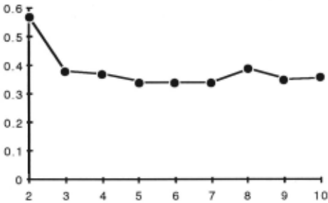
In our experiments, we attempted solutions with different values of m, the maximum number of pseudo-classes, and reported results for the value of m that gave the best goodness of fit. The dependence of goodness of fit on the value of m is illustrated in Figure 7 which plots the relative error vs. the number of pseudo-classes for the sinormal data.
| Dataset | Tree Size | Tree Error | Rule Size | Rule Error |
|---|---|---|---|---|
| Sine | 200 | .03 | 76 | .02* |
| Normal | 63 | .II | 18 | .08* |
| Sinormal | 16 | .49 | 6 | .34* |
| Iris | 9 | .22 | 8 | .22 |
| Drug Study | 7 | .40 | 5 | .38 |
| Whitecap | II | .71 | 2 | .67 |
| Heart | 6 | .82 | 4 | .82 |
This is a prototypical plot of complexity vs. goodness of fit that can be seen in the other applications. As the number of partitions increases, results improve until they reach a relative plateau and deteriorate somewhat. Similar complexity plots can be found for other models, for example neural nets [Weiss and Kapouleas, 1989].
4 Discussion
In our experiments, the regression rules generally outperformed the regression trees. Fewer constant regions were required and the estimated error rates were generally lower. An estimator such as GCV (described in equation 6) which combines both complexity and performance, is likely to accentuate the advantage of regression rules. Finding these DNF regions was substantially more computationally expensive for the regression rules than the regression trees. For the regression rules, fairly complex optimization techniques were necessary. In addition, experiments must be performed to find the appropriate number of pseudo-classeo;; . Of course, this is more a matter of scale: scale of the application versus the scale of available computing. Of the applications considered, no application takes more than I5 minutes of cpu time on a RS6000/320H for a single pseudo classification problem and a full cross-validation. 5 As computing power increases the timing distinction is less important. Even a small percentage gain can be quite valuable for the appropriate application [Apte, Weiss, and Grout. 1993] and computational requirements are a secondary factor.
5 A 10-fold cross-validation requires solving a problem essentially II times: once on all training cases and 10 times for each group of test cases.
In this paper, we considered a new model for rule-based regression and provided comparisons with tree-based regression. However, these results must be considered preliminary. Because most of the datasets were nonlinear, classical linear statistical models should do poorly. We have not performed any comparisons with alternate nonparametric models of regression, such as projection pursuit, neural nets or nearest neighbor methods. However, independent of alternate models, the advantages of strong explanatory capabilities and high dimensional feature selection can make a DNF model the model of choice in many applications. This is particularly true for knowledge based applications, for example equipment repair or medical diagnosis, in contrast to pure pattern recognition applications such as speech recognition.
We have presented the regression problem with one output variable. This is the classical form for linear models and regression trees. The issue of multiple outputs bas not been directly addressed although such extensions are feasible. This issue and further experimentation await future work. Our model of regression can provide a basis for these efforts, while leveraging current strong methods in classification rule induction.
Acknowledgments
We acknowledge the support of our colleagues at the IBM TJ Watson Research Center (Math Department) and A TT Bell Laboratories. Most helpful were discussions with C. Apte of IBM and V. Seshadri of Bell Labs. We are also grateful for the financial support provided by Telecom Australia Research Laboratories.
@inproceedings{ijcai1993p148,
  title     = {Rule-Based Regression},
  author    = {Weiss, Sholom M. and Indurkhya, Nitin},
  booktitle = {Proceedings of the Thirteenth International Joint Conference on
               Artificial Intelligence, {IJCAI-93}},
  publisher = {International Joint Conferences on Artificial Intelligence},
  editor    = {Ruzena Bajcsy},
  pages     = {1072--1077},
  year      = {1993},
  note      = {Machine Learning},
  url       = {https://ijcai.org/proceedings/1993/148},
}
TY - CPAPER TI - Rule-Based Regression AU - Weiss, Sholom M. AU - Indurkhya, Nitin T2 - Proceedings of the Thirteenth International Joint Conference on Artificial Intelligence, IJCAI-93 PB - International Joint Conferences on Artificial Intelligence PY - 1993 SP - 1072 EP - 1077 UR - https://ijcai.org/proceedings/1993/148 ER -Copied
Machine-readable versions of this paper, for tools and AI agents:





