
Complex Concept Acquisition through Directed Search and Feature Caching
Proceedings of the Thirteenth International Joint Conference on Artificial Intelligence. Machine Learning. Pages 946-950.
© 1993 International Joint Conferences on Artificial Intelligence
Abstract
Difficult concepts arise in many complex, formative, or poorly understood real-world domains. High interaction among the data attributes causes problems for many learning algorithms, including greedy decision-tree builders, extensions of basic methods, and even backpropagation and MARS. A new algorithm, LFC, uses directed lookahead search to address feature interaction, improving hypothesis accuracy at reasonable cost. LFC also addresses a second problem, the general verbosity or global replication problem . The algorithm caches search information as new features for decision tree construction. The combination of these two design factors leads to improved prediction accuracy, concept compactness, and noise tolerance. Empirical results with synthetic boolean concepts, bankruptcy prediction and bond rating show typical accuracy improvement of 15%-20% with LFC over several alternative algorithms in cases of moderate feature interaction. LFC also explicates latent relationships in the training data to provide useful intermediate concepts from the perspective of domain experts.
- [Breiman et al., 1984] L. Breiman, J. Friedman, R. 01- shen and C. Stone. Classification and Regression Trees . Wadsworth, Belmont, CA, 1984.
- [Fu and Buchanan, 1985] L.-M . Fu and B.G. Buchanan. Learning intermediate concepts in constraining a hi- erarchical knowledge base. In Proc. Ninth Inti. Joint Conf. on AI, 659-666, 1985.
- [Ginsberg and Harvey, 1992] M.L. Ginsberg and W .D. Harvey. Iterative broadening. Artificial Intelligence, Vol.55, No.2-3, 367-383, June 1992.
- [Gentry et al., 1990] J .A. Gentry, P. Newbold and D.T . Whitford. Profiles of cash flow components. Finan- cial Analysts, 41-48, July-August 1990.
- [Mehlsam, 1989] G. Mehlsam. Automatisches Erzeugen von Klassifikationskriterien. Doctoral Dissertation, Technische Universitat Wien, Austria, 1989.
- [Norton, 1989] S. Norton. Generating better decision trees. In Proc. Eleventh Inti. Joint Conf. on AI, 800-805, 1989. IJCAI
- [Pagallo, 1990] G. Pagallo. Learning DNF by decision trees. Ph.D. Thesis, University of California at Santa Cruz, 1990. IJCAI
- [Ragavan and Rendell, 1991] H. Ragavan and L.A. Ren- dell. Relieving limitations of empirical algorithms. In Proc. Change of Representation Workshop. Twelfth Inti. Joint Conf. on AI, 1991.
- [Ragavan and Rendell, 1993] H. Ragavan and L.A. Ren- dell. Lookahead feature construction for learning hard concepts. In IProc. Tenth Inti. Machine Learn- ing Conf., 1993.
- [Rendell and Ragavan, 1993] L.A. Rendell and H. Raga- van. Improving the design of induction methods by analyzing algorithms functionality and data-based concept complexity. In Proc. Thirteenth Inti. Joint Conf. on AI, 1993 (this volume) .. sp .5
- Shaw and Gentry] M.J. Shaw and J.A. Gentry. Induc- tive learning for risk classification. IEEE Expert, 47- 53, February 1990.
References were extracted automatically from the PDF and may contain errors.
Full text extracted automatically from the PDF; figures, tables and equations may differ. The PDF is the version of record.
1 Introduction
We describe a learning method for complex concepts and practical results in the difficult financial domain of risk classification. Financial data are collected in the form of observations and an overall assessment (often binary-to lend or not to lend). This constitutes an attribute-value representation, where each training example is described by an n-tuple of attribute values and a class value. A concept is an intensional description of the class; a learn ing algorithm constructs a hypothesis of the concept. Learning that assumes class-membership varies little as hypothesis descriptions are modified slightly has been called similarity-based (SBL).
·This work was supported in part by NSF grant IRI-9204473, a KPMG Peat Marwick Foundation award, a Unive~ sity of Illinois Research Board award, and a Beckman Insti tute Cognitive Science and Artificial Intelligence Fellowship.
Shaw and Gentry (1990] have shown advantages of SBL over traditional financial classification methods such as discriminant analysis. Some statistical ap proaches allow nonlinearity, but SBL is more readily comprehensible and facilitates human-computer interac tion. While many concepts pose no problems for typical decision tree induction algorithms, complex domains of ten produce inaccurate trees. As shown later, C4.5 give low predictive accuracies for finacial concepts. Other methods such as improved SBL and backpropagation also fare poorly.
Financial risk classification is difficult because of in teraction among the attributes. In a critique of current learning systems, Rendell and Ragavan [1993, this vol ume] examine relationships among attribute interaction, real-world problems, and system requirements.
This paper explores a new algorithm called LFC (lookahead feature construction) which applies directed lookahead search to build decision trees and form new features . LFC uses several techniques to decide dynam ically which paths to attempt, how far to pursue the search, and which new features provide the most concise hypothesis components.
Section 2 details the algorithm. Section 3 reports ex periments comparing LFC with other methods, using controlled synthetic data, a bankruptcy concept, and a bond rating concept . On complex concepts, LFC is rea sonably fast and much more accurate. In Section 4 we also consider the value of the new feature constructions to a financial expert. Consistent constructions support and extend the expert's own notions to promote a reli able model of the domain.
2 The LFC Algorithm
LFC (Fig. 1) constructs new features using the ID3 in formation gain function ci> . Its novelty lies in using a geometric representation for beam search with branch and bound (Sees. 2.1 & 2.2). The algorithm handles discrete-valued data representations, such as integers, booleans, and nominals. For continuous-valued represen tations (reals), LFC first intervalizes the data attributes, based on minimizing the class entropy in each interval (or on user-specified intervals). Noisy training samples are handled through feature pruning and tree pruning.
Given: A set of original attributes Foriginal, beam features Fbeam, window width A, and training examples Dtrain·
Returns: A set of new features, Fnew.
- Select the best feature /be·t from Fbeam . Remove original attributes lying at a distance greater than A from but in S, retaining only F~riginal s;; Foriginal·
- Select an attribute x from F~riginal that is not al ready present in Fbeam. Let /original = either x or -.x, whichever maps closer to (Pma:r, 0).
- Try to construct a new feature !new = b ·· t 1\ /original · IF !new is worse than either but or !original then discard /new. ELSE Fnew := Fnew U /new·
- Remove /but from Fbeam and repeat steps 1-4 until Fbeam = 0.
Given: A set of original attributes Foriginal, beam size a, maximum search depth I, stopping sample size /3, and training examples Dtrain·
Returns: A decision tree with new features.
IF !Dtrainl < /3 or all the examples in Dtrain are of the same class, create a leaf node. If the majority of examples in Dtrain is positive, label the leaf as positive, otherwise negative. ELSE
- Fnew := Foriginal·
- Select the a best features for the beam, Fbeam s;; Fnew· Call FC to construct new features Fnew from Fbeam and Foriginal·
- IF no feature in Fnew is better than any feature in Fbeam, or if the limit I is reached, then stop the beam search.
ELSE Repeat steps 2 and 3.
- Select the feature with the lowest \II from Fbeam and prune it. Call this fbe.t ·
- Create a new decision-tree node corresponding to J; ·· ,.
- For each partition block II from splitting Dtrain us ing fbe·t ' set Dtrain := II and recursively call LFC.
Figure 1: Pseudocode for FC (top) and LFC (bottom) Algorithms.
LFC first selects a subset of a attributes from the n original attributes for the beam. These a features are used as operands. The beam features are initially selected from the original attributes, and subsequently from both the original attributes and the constructed features. After a maximum search depth of I levels, the "best" (highest ~) feature is selected for the decision node.
The feature construction operators are negation and conjunction, although disjunction may also be used. If all three operators are given, FC chooses either conjunc tion or disjunction, whichever is better, to avoid repeat ing semantically equivalent features, since by DeMor gan 's law, the set { -., 1\} is functionally complete.
The constructed feature is pruned back by evaluat ing the number of misclassifications by the feature on an independent test sample [Breiman et al., 1984]. The last (usually least significant) attribute in the feature (which is a conjunction of attribute literals) is iteratively dropped, until either the error is minimized, or until a single attribute is left.
After constructing a new feature for a decision-tree node, LFC splits the data and iterates on each partition block, until either a specified mix of positive and neg ative examples or a minimum sample size for splitting is reached (stopping criterion) . The tree is then pruned back based on test sample error minimiz.ation.
2.1 Constraining Construction Geometrically
A key to guiding feature construction search is to relate the ~ value of a feature to the individual ~ values of its component attributes. Normally this relationship is not explicit, and it is possible for two low ~ attributes to produce a high ~ feature when conjoined. In this section, we introduce a mapping technique for making this relationship more explicit.
The information gain~ of an attribute (or constructed feature) depends only on the number of positive and negative examples after splitting the data using the at tribute, rather than on the exact examples themselves. <I> increases when the mix of positive and negative ex amples in each partition block decreases, and is maxi mum for partition blocks comprising purely positive and negative examples. The best features thus have high ~ values.
Mapping each data attribute or new feature based on the counts of positive and negative examples covered by the attribute gives a geometric representation of their quality. A similar study using ~ values was discussed by Mehlsam [1989], although his algorithm for constructing features moves objects from one partition block to an other in a greedy manner, like the scheme of Breiman et al. [1984] . In contrast, LFC maps the original at tributes to a geometric representation, then applies beam search and branch-and-bound directly using this repre sentation. This technique applies lookahead search, fo cused by natural constraints arising in the representation to prune off large chunks of the search space. The follow ing section details these new techniques to guide feature construction.
2.2 Mapping Features by Utility
Let Pmax and Nmax be the total number of positive and negative examples in the training data. In Figure 2, S is the plane bounded by (0, 0) and (Pmax, Nmax) with axes P and N . The line B given by ((0, 0), (Pmax, Nmax)) bi sects S into a lower half-plane L and an upper half-plane U. Initially, every original attribute-value x is mapped to a point (p, n) on S, where p and n are the number of positive and negative examples covered by this attribute value. Subsequently, the beam features are also mapped to S. We use p( x) to indicate the point (p, n) on S corre sponding to x, where xis an original attribute or a new feature.
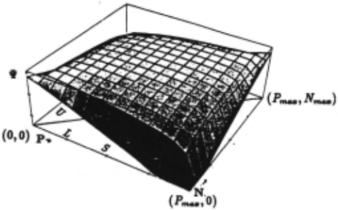
The information gain of xis given by <I>(x) = H -llt(x ), where llt(x) is conditional entropy and H is prior class entropy. Maximizing <I> minimizes Ill, since H remains constant at every stage of decision-tree building. In Fig ure 2, llt(x) is expressed as a function of the number of positive and negative examples covered by x, p and n respectively. Ill is maximum at points along B; these points correspond to features with zero discriminatory power. In L, Ill decreases monotonically along any line parallel to P and increases monotonically along any line parallel to N; it shows similar behavior in U. Ill has the minimum value 0 at (Pma:z:, 0). A hypothesis covering all the positive examples and excluding all the negative examples maps to the extremity of S given by (Pma:z:, 0). Features corresponding to conjunctive terms of the con cept C map to points on P, whereas terms of its com plement C map to points on N.
2.3 Construction Using Branch-and-Bound
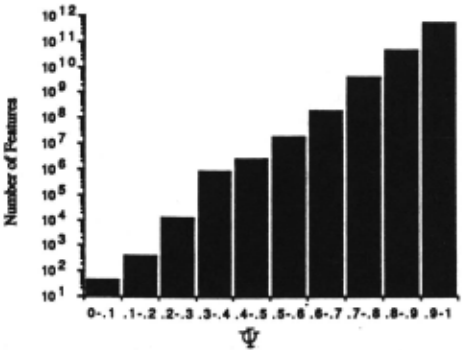
Figure 3 shows the frequency of occurrence of all possible features in S (log-scale) lying within a particular range of Ill values. Most features have high Ill values, and the frequency of feature occurrence diminishes exponentially as 'lit reduces. Suppose an original attribute has a Ill value of 0.3 in Figure 2. It is sufficient to search for features to the left of 0.3, since the worst we can do is 0.3. The problem is how to analyze the features to make this search feasible.
Consider where the features map in Figure 2. Ill is high along B, going down as we move toward P (or N). Fo cusing search on features lying in a neighborhood around the original attribute and between the P axis eliminates most of the high entropy features close to B. FC ap plies a "window" filter around an operand x, to filter points lying too far away from p( x) or P (a parameter >., 0 < >. S 1 specifies the relative width of the window). The beam attributes mapping outside this window are removed, and only those inside the window are used for construction. This neighborhood contains far fewer fea tures than the space of all possible features, making it is easier to find good features that lie in the range 0 to 0.3.
Nevertheless, the number of features could still be large; this is tackled by brand-and-bound search. FC chooses a feature from . the beam as one of its two operands; for its second operand, FC selects an origi nal attribute value closest to (Pma:z:, 0). Suppose these two component attribute values x1 at (p1, nl) and x2 at (p2, n2) produce the feature It = x1 1\ x2. The number of positive (or negative) examples covered by It can at most be Pl (n!) or P2 (n2), whichever is lower. Therefore p(ft) lies inside the rectangle of intersection R1 given by ((O,O),(min(pl,P2),(min(nl,n2)). The lowest value of Ill inside R1 occurs either at (min(pl,P2), 0) or at (0, min(n1 , n2)). If this value is higher than the value at (PI, nl) or (p2, 112), then the best (lowest) value of Ill for ft is worse (higher) than the 'lit values at x1 or x2. This indicates that It is worse than the better of x1 or x 2 , so It is eliminated. (A dual technique may be used for eliminating x1 V x2 .) Moreover, all features formed from conjunctions of ft may be dropped because of this prop erty. At every step of the beam search, if no new feature is better than the existing ones, feature construction is stopped, even before the search depth of l is reached, au tomatically terminating search early. Choosing the best a attributes for the beam corresponds to choosing the steepest a gradients on the Ill surface. Starting from a point p( x) on S corresponding to an original attribute x, FC produces new features mapping to points that move closer toward P, eventually stopping at P.
3 Empirical Analysis
We compare several algorithms with LFC. In addition to hypothesis predictive accuracy, the performance criteria also include speed, which we omit in this short version of the paper (LFC speeds are competitive). Our use of feature construction suggests other criteria, such as consistency and comprehensibility, factors that promote useful expert-system interaction. The algorithms we tested are standard SBL methods (JD3, C4.5, and PLS), various SBL improvements (GREEDY3, FRINGE, and LFC) , and also backpropagation (BP). We first consider synthetic data to allow control of attribute interaction. Next, we present results in two difficult financial do mains. Results for these domains appear in in three respective subsections. (Ragavan & Rendell [1993] give other results) .
3.1 Comparisons Using Synthetic Concepts
As a preliminary assessment for LFC and two other methods, we use controlled attribute interaction in boolean concepts. An mjn parity concept is an m-bit boolean parity function described with training examples using n bits (m ~ n). For fixed n , attribute interaction increases as m increases; the concept becomes more dif ficult to learn because the number of training examples is the same for all the concepts.
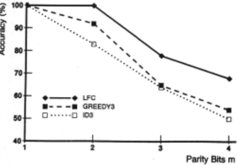
Figure 4 shows results with three algorithms when learning m/7 parity concepts. For different m, Figure 4 shows predictive accuracy. GREEDY3 uses depth-first search for greedy feature construction to construct de cision lists (Pagallo, 1990) . Each point in Figure 4 was obtained by averaging over 10 runs, using independent training and testing sets. Each algorithm was trained us ing 55 examples , and tested using 72 unseen examples. In each run, the tree was inconsistent with at most 4 out of 48 training examples.
Figure 4 shows that LFC produces more accurate trees compared with ID3 and GREEDY3. As m increases, attribute interaction increases, so the average predictive accuracy decreases for all three algorithms because of the sparse training sample. Although the rate at which all algorithms degrade may be controlled by adjusting the size of the training sample, the sample size was held constant to study this degradation with higher attribute interaction. This gives the fairly high degradation rate observed in Figure 4, but LFC still maintains higher accuracy, and shows slower degradation than the other algorithms.
We also investigated the behavior of LFC and other methods using complex financial problems: bankruptcy prediction and bond rating. The next two sections de tail these results. The data attributes were developed by experts using cash-flow theories, and represent situ ations of real companies. The last two authors of this paper have found that LFC constructed features that are identifiable and significant from the domain perspective.
| I Algorithm | I Accuracy (%) |
| GREEDY3 | 58.0 ± 7.0 |
| PLS | 64.9 ± 0.4 |
| FRINGE | 65.9 ± 0.6 |
| C4.5 | 70.0 ± 5.4 |
| Backprop | 76.1 ± 3.8 |
| LFC | 90.1 ± 0.4 |
3.2 Comparisons Using Bankruptcy Data
Numerous empirical models have been developed that use annual financial information discriminate firms that declare bankruptcy from these that remain solvent. Lenders and investors want to improve their ability to explain, interpret , and predict bankruptcy. Our study used 198 bankruptcy data; half of the companies went bankrupt in a given period while the other half were fi nancially healthy during the same time period. A cash flow model was used to define the fifteen attributes, which include net operating flow (NOF), financial costs (NFC), and change in inventory (INVF) [Gentry et al., 1990] .
3.2.1 Prediction Accuracy
Table 1 shows results with the bankruptcy data, which was randomly split into mutually exclusive training and testing sets containing 95% and 5% of the examples re spectively. Table 1 compares the predictive accuracy of LFC with that of five other algorithms. Each accuracy figure was obtained by averaging over several runs (50 in most cases) using mutually exclusive training and test ing sets. The means are shown with 99% confidence intervals.
PLS and FRINGE gave 65% and 66% accuracy, com parable to the prior class frequency estimate of 49.7%. GREEDY3 produced an accuracy of 58%. Possibly be cause of tree pruning, C4-5 gave a much better accuracy of 70%. However, the variability in the accuracy of its trees is high(± 5.4%). Consequently, the improvement is not significant at p < 0.001, t-test. We also tested backpropagation with many parameter settings and net structures. The best choice was 14 input nodes, 8 in termediate nodes, and 1 output . The best accuracy we could obtain was 76%.
In contrast , LFC gave an average accuracy of about 90%, improving over each of the other algorithms (p < 0.001, t-test) . Tree variability was very low (± 0.4%) . We measured t.he relationship of accuracy to the amount of lookahead used by LFC. The lookahead depth was varied from 1 to 3. The accuracies were, respectively,
64%, 84%, and 90% (99% confidence intervals were ± 1.7 for I = 1, 2, and ± 0.4 for I = 3). With no looka head, LFC's performance approaches that of PLS. As lookahead depth increases, LFC makes more informed selections for a decision node, improving accuracy and consistency.
3.2.2 Discovering Meaningful Features
In our experiments with the bankruptcy data, LFC re duced verbosity and compressed the decision tree from 10 nodes for PLS to 7 nodes on the average. LFC also improved the abstraction of the decision trees by dis covering new financial concepts, which capture specific risk characteristics of a company (shown in Table 2). One example from Table 2 is inventory financing IN F I, which relates the change in inventory (!NV F) to the fixed coverage expenditures (FCE), and the flows from operations (NOF). IN F I abstracts the three low level attributes NOF, FCE, and !NV F. This feature is an intermediate concept [Fu and Buchanan, 1985] charac terizing the company's strategy to finance its inventory. IN F I is true for companies that need to finance an in crease in inventory but avoid financing with long-term debts; Table 2 summarizes the features that occurred most frequently in six typical trees for the bankruptcy concept. Each feature is expressed in terms of both the original attributes it relates and also its corresponding real-world concept.
3.3 Comparisons with Bond Rating Data
Bond ratings are used in the capital market as yardsticks for estimating potential yields. The bond rating data set had 125 samples, and three classes. The concept gave an average accuracy of 42% with C4.5 for all three classes. No other comparison algorithm did better, except back propagation, which achieved 50% as the best of many varied trials. LFC (extended for multiple classes) did considerably better, with an average accuracy of 70%.
For the first class (high risk bonds), the average pre dictive accuracy of the LFC trees was 83%. The av erage size was 20 decision nodes. In all, 14 boolean conditions using the original attributes were generated. Because each new feature could contain up to three original attributes, the feature search space contained 14 x 13 x 12 = 2184 possible features per node. This figure is the total number of choices, i.e., the number in 3-ply exhaustive and naive lookahead.
In contrast, LFC evaluated only 755 features, which is about 38 features/node, an enormous reduction from 2184. Hence LFC searches less than 2% of the feature space. Of these 755 features, LFC selected 20 for the final nodes of the decision tree.
In terms of accuracy, exhaustive lookahead is the only competitor of LFC. Although LFC is slower than some methods, its times are reasonable, especially in the light of the many hours required for exhaustive lookahead (we compared LFC in full search mode and also Bun tine's IND). Other techniques, including backpropaga tion, were little or no faster, and produced significantly and considerably inferior hypotheses. LFC is also supe rior with respect to human comprehension and expert computer interaction.
4 Discussion
A typical divide-and-conquer splitter (e.g., CART, Breiman et al., 1984) iteratively partitions the data us ing the single best attribute to create a decision node. Although this greedy procedure is efficient, it may get trapped by local optima and degrade the quality of the induced decision tree [Ragavan and Rendell, 1991]. This occurs when the concept has a high degree of attribute interaction [Rendell and Ragavan, 1993, this volume]. Attribute interaction increases the number of original at tributes ( conjuncts) required to specify meaningful sub classes at the leaves. Attribute interaction also causes node replication [Pagallo, 1990], which degrades accu racy, consistency, and comprehensibility.
Some algorithms have extended greedy splitters; e.g., FRINGE [Pagallo, 1990] uses the decision tree produced by a greedy splitter to construct new features for improv ing tree quality. Repeated fringe patterns near the leaves of the tree are coalesced to give new features, which are combined with the original attributes to build a new de cision tree. The process iterates. But such strategies are insufficient when attributes interact much. This is be cause the original decision tree is greedy and because re peated decision patterns are distributed throughout the tree, rather than being confined to fringes. Replications become complex and glo.bal.
One way to extend SBL splitters is to look ahead to observe the effects of current attribute selection further down in hypothesis construction. The best sequence may be found when all possible expansions of a decision tree are evaluated. This avoids problems of attribute interac tion. Norton [1989] found fairly good improvement with an exhaustive lookahead algorithm IDX, though it does not construct new features to cache the search knowl edge. While splitters can construct better hypotheses with fulllookahead search, naive lookahead search is ex pensive, and unnecessary in many cases.
A practical cure for attribute interaction is dynamic lookahead. LFC constructs features while building the decision tree. LFC can replace a greedy algorithm for the decision tree construction phase of FRINGE-like al gorithms, but it largely prevents tree patterns from re peating in the first place. A sequence of decisions down any path of a decision tree is treated as a conjunction of attributes for constructing a new feature. The fea tures are not evaluated individually, but instead as a group, effectively projecting multi-dimensionally [Raga van and Rendell, 1991]. Forming a new feature from the attributes economically caches this search information.
LFC guides lookahead search and feature construc tion by taking advantage of patterns in the training data and natural search constraints that arise in its geomet ric search representation. The algorithm deepens search only when necessary, stopping when it reaches the P axis (Fig. 2). The window filter is used for initial selection of candidate original attributes for feature construction, based on their quality. Subsequently, the beam is cho sen based upon where the features and attributes map in the geometric plane. Variable beam width is a type of iterative broadening [Ginsberg and Harvey, 1992]. The distinction in LFC is the way it focuses on essential parts of the search space and prunes irrelevant parts with its branch-and-bound. FC uses only the coordinates of the component attributes to determine whether to eliminate new features constructed from them, so the data are not split on a feature that may be discarded, or conjunc tions thereof. Ragavan and Rendell [1993] present other comparative results using LFC.
| Feature Details | Intermediate Concept |
|---|---|
| INVF"' ~ 0 and FCE"' ~ 0 or INVF* < 0 and NOF* > .2 AD/FA< .67 and ARF* > .5 or AD/FA ~ .67 and safe inventory financing NOF* $ .2 or (AD/FA$ .33 and NOF* $ .33) or NOF* > .2 and AD/FA> .5 OCAF* > -.13 and OCLF* < -.2 or OCAF* < -.13 and NFF*-< 0 NOF* < -:-33 and FCE* < 0 or FCE* -< -0.2 or AD/FA< 0 | safe inventory financing impact of maturity of the firm on current asset management experience of the company in operating efficiently debt repayment strategy long-term financial strategy |
New features help to build a high-level knowledge structure for more accurate and comprehensible mod els. An important issue is closer interaction between the learning algorithm and the domain expert. In the complex financial domains of Section 3, the higher-level hypotheses produced by LFC facilitate interpretation of results and help to refine important attribute relation ships.
5 Conclusions
Severe attribute interaction in real-world domains makes learning hard for similarity-based and other induction al gorithms. We analyzed a global search technique for fea ture construction that improves learning for controlled synthetic and difficult natural financial domains. Accu racy improves by as much as twenty percentage points. Interpretation of the new features and decision trees by domain experts corroborates improvement in their ab straction. Repeatability of the constructed features im proves expert-machine interaction.
In LFC the complexity of feature construction is re duced by a combination of analytic and heuristic tech niques. The algorithm is distinctive because it tackles both the attribute interaction problem (using directed lookahead) and the global replication problem (through feature construction). Rendell and Ragavan [1993, this volume] detail these phenomena.
LFC improves learning in several respects:
- Predictive accuracy of decision trees
- Consistency of the trees, measured by the variance in their predictive accuracy
- Reduction in the complexity of lookahead search for feature construction, through a geometric procedure
- Significance of the tree nodes (features) from a domain perspective.
@inproceedings{ijcai1993p130,
  title     = {Complex Concept Acquisition through Directed Search and Feature Caching},
  author    = {Ragavan, Harish and Rendell, Larry A. and Shaw, Michael J. and Tessmer, Antoinette},
  booktitle = {Proceedings of the Thirteenth International Joint Conference on
               Artificial Intelligence, {IJCAI-93}},
  publisher = {International Joint Conferences on Artificial Intelligence},
  editor    = {Ruzena Bajcsy},
  pages     = {946--950},
  year      = {1993},
  note      = {Machine Learning},
  url       = {https://ijcai.org/proceedings/1993/130},
}
TY - CPAPER TI - Complex Concept Acquisition through Directed Search and Feature Caching AU - Ragavan, Harish AU - Rendell, Larry A. AU - Shaw, Michael J. AU - Tessmer, Antoinette T2 - Proceedings of the Thirteenth International Joint Conference on Artificial Intelligence, IJCAI-93 PB - International Joint Conferences on Artificial Intelligence PY - 1993 SP - 946 EP - 950 UR - https://ijcai.org/proceedings/1993/130 ER -Copied
Machine-readable versions of this paper, for tools and AI agents:





