
Learning DNF by Decision Trees
Proceedings of the Eleventh International Joint Conference on Artificial Intelligence. Machine Learning. Pages 639-643.
© 1989 International Joint Conferences on Artificial Intelligence
Abstract
We investigate the problem of learning DNF concepts from examples using decision trees as a concept description language. Due to the replication problem, DNF concepts do not always have a concise decision tree description when the tests at the nodes are limited to the initial attributes . However, the representational complexity may be overcome by using high level attributes as tests. We present a novel algorithm that modifies the initial bias determined by the primitive attributes by adaptively enlarging the attribute set with high level attributes. We show empirically that this algorithm outperforms a standard decision tree algorithm for learning small random DNF with and without noise, when the examples are drawn from the uniform distribution.
- [Blumer et al., 1987] A . Blumer, A . Ehrenfeucht, D. Haussler, and M. Warmuth . Occam's razor. In- formation Processing Letters, 24:377-380, 1987.
- [Breiman et al., 1984] L. Breiman, J .H. Friedman, R.A. Olsen, and C.J. Stone. Classification and Regression Trees. Wadsworth Statistic/Probability Series, 1984.
- [Haussler, 1988] D. Haussler. Quantifying inductive bias: AI learning algorithms and Valiant's learning framework. Artificial Intelligence, (36):177-221, 1988.
- [Michalski, 1983] R. Michalski. A theory and method- ology of learning. In Machine Learning: An Artificial Intelligence Approach, pages 83-134.
- Morgan Kauf- mann, 1983.
- [Muggleton, 1987] S. Muggleton. Duce, an oracle based approach to constructive induction. In Proc. IJCAI- 87, pages 287-292 . IJCAI
- Morgan Kaufmann, 1987.
- [Pagallo and Haussler, 1988] G. Pagallo and D . Haus- sler. Feature discovery in empirical learning. Tech- nical Report UCSC-CRL-88-08, Dept . of Comp . Sci- ence, Univ. California, Santa Cruz, 1988.
- [Quinlan, 1986] J .R. Quinlan. Induction of Decision Trees. Machine Learning, 1:81-106, 1986.
- [Quinlan, 1987a] J .R. Quinlan. Generating production rules from decision trees. In Proc. IJCAI-87, vol- ume 1, pages 304-307. IJCAI
- Morgan Kauffman, 1987.
- [Quinlan, 1987b] J .R. Quinlan. Simplifying decision trees. International Journal of Man-machine Studies , 27:221-234, 1987.
- [Rivest, 1987] R. Rivest. Learning decision lists . Ma- chine Learning, 2:229-246, 1987.
- [Schlimmer, 1986] J. C. Schlimmer. Concept acquisition through representational adjustment. Machine Learn- ing, 1:81-106, 1986.
- [Subutai and Tesauro, 1988] A. Subutai and G. Tesauro. Scaling and generalization in neu- ral networks: A case study. In Proc. IEEE-88 Conf. on Neural Inf. Proc. Systems-Natural and Synthetic, 1988.
- [Utgoff and Mitchell, 1982] P. Utgoff and T . M. Mitchell. Acquisition of appropriate bias for inductive concept learning. In Proc. AAAI-82, pages 414-417.
- Morgan Kaufmann, 1982.
- [Valiant, 1985] L. G. Valiant. Learning disjunctions of conjunctions. In Proc. IJCAI-85, pages 560-566.
- Mor- gan Kaufmann, 1985.
- [Vapnik, 1982] V. N. Vapnik. Estimation of Dependen- cies Based on Empirical Data. Springer Verlag, 1982.
- [Wilson, 1987] S. W . Wilson. Classifier systems and the animat problem. Machine Learning, 2:199-228, 1987.
References were extracted automatically from the PDF and may contain errors.
Full text extracted automatically from the PDF; figures, tables and equations may differ. The PDF is the version of record.
1 Introduction
The goal of a system that learns from examples is to improve classification performance on new instances of some target concept, after observing a relatively small number of examples. A key technique is to formulate a simple explanation (hypothesis) of the training examples using a concept description language. Then, a new in stance is classified according to the induced hypothesis.
The simplest way to describe an instance is by a mea surement vector on a set of predefined attributes. An attribute comprises a (possibly) relevant characteristic of the target concept, and an attribute measurement re veals the state of the attribute in the observed instance. Such description is called attribute-based.
A frequently studied class of target concepts in attribute-based learning is the class of target concepts that can be represented by small Disjunctive Normal Form (DNF) formulae [Valiant, 1985, Haussler, 1988, Michalski, 1983]. While general purpose learning algo rithms have been proposed for certain subclasses of sim ple DNF formulae [Valiant, 1985], the general problem is still open. In this paper, we investigate the problem of learning small DNF concepts using decision trees as the concept representation language [Breiman et al., 1984, Quinlan, 1986].
Concepts with a small DNF description do not al ways have a concise decision tree representation when the tests at the decision nodes are limited to single at tributes. The representational complexity is due to the fact that the tests to determine if an instance satisfies a term have to be replicated in the tree. We call this rep resentational shortcoming the replication problem. The problem is reduced (and, eventually disappears), as we show in Section 3, by using high level attributes as tests in the tree. The complexity of classification rules derived from decision trees have been also addressed in [Breiman et al., 1984, Quinlan, 1987b].
For learning, appropriate high level attributes may be defined a priori or dynamically by the learning al gorithm. When the features are defined a priori, they are usually determined as combinations of the primi tive attributes of a fixed type and size, e.g., conjunctions up to a fixed size [Breiman et al., 1984, Valiant, 1985, Rivest, 1987]. In general, only a small number offeatures defined are meaningful for learning. A higher percent age of relevant features can be obtained, for example, by using knowledge about the concept at hand.
On the other hand, when the features are defined by the learning system, no background knowledge about the target concept is needed. The capability of a learning algorithm to enlarge adaptively the initial attribute set is called dynamic bias [Utgoff and Mitchell, 1982]. General purpose learning systems with this capability have been proposed, for example, in [Schlimmer, 1986, Muggleton, 1987].
In this paper, we present a novel heuristic for a deci sion tree algorithm to modify the initial bias determined by the primitive attributes by dynamically introducing high level attributes. The learning algorithm we present (called FRINGE), builds a decision tree using the primi tive attributes, and analyses this tree to find candidates for useful features. Then, it redescribes the examples using the new attributes, in addition to the primitive at tributes, and builds a new decision tree. This process is iterated until no new candidate attributes are found.
The performance of FRINGE was tested in several synthetic Boolean domains. Our results show that FRINGE improves upon the classical decision tree ap proach when the target concept has a small DNF de scription, even in the presence of noise. However, when a target concept has no small DNF description, (e.g., the majority function) or when the attribute values are not correlated to the classification (e.g., the parity func tion), FRINGE cannot improve significantly on the poor performance of the classical approach.
2 Definitions
In this section we introduce the notation and definitions that formalize the basic notions we use in this paper. To simplify our presentation we limit ourselves to the case where all attributes are Boolean.
A decision tree is a tree with labelled nodes and edges. In our setting, an internal node defines a binary test on an attribute. For example, the root node of the tree in Figure 1 defines the test is "x1 = 1 ?". Each edge represents an outcome of the test. We use the convention that the left edge represents the negative outcome, and the right edge represents the positive outcome. The label of a leaf represents the class label that is assigned by the tree to any example that reaches this node.
The size of a concept description with respect to a representation language is the number of bits required to write down the description. For simplicity, we mea sure the size of a decision tree by the number of internal nodes.
Finally, we introduce some terminology to refer to combinations of Boolean attributes. A literal is an at tribute or its complement. A term is a conjunction of literals, a clause is a disjunction of literals. In general, a feature is any Boolean combination of the attributes obtained by applying Boolean operators to the primitive attributes. We use the term variable to refer to a prim itive attribute or to a feature. We use ·, + and- (bar) to denote the Boolean operators and, or and not respec tively.
3 Decision trees
The common procedure to learn a decision tree from ex amples is based on successive subdivisions of the sample. This process aims to discover sizable subsets of the sam ple that belong to the same class. The tree structure is derived by a top-down refinement process on the sample.
Initially, we begin with an empty decision tree and a sample set. A test is applied to determine the best attribute to use to partition the sample. Following [Breiman et al., 1984, Quinlan, 1986] , we measure the merit of an attribute with respect to the subdivision pro cess by the mutual information between the class and the attribute. Then, the best attribute according to this measure is placed at the root of the tree, and the ex amples are partitioned according to their value on that attribute. Each subset is assigned to one subtree of the root node, and the procedure is applied recursively. The subdivision process on one branch of the tree ends when no attribute provides information about the class label i.e., every attribute has zero mutual information. Thi~ leaf is labelled with the common class of these examples.
To avoid overtraining, the tree grown by the subdivi sion process described above is pruned back. We use the Reduce Error Pruning method proposed by Quinlan in [Quinlan, 1987b].
4 The replication problem
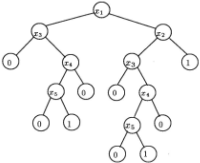
A decision tree representation of a Boolean function with a small DNF description typically has a peculiar struc ture: the same sequence of decision tests leading to a positive leaf is replicated in the tree. To illustrate the problem, consider the Boolean function x 1 -x2+x3 -x4 -x5 .
The smallest decision tree for the function has the fol lowing structure (see Figure 1): Each decision test in the rightmost path of the tree is an attribute of the shortest term in the formula. The path leads to a positive leaf and it corresponds to the truth setting for the first term. The left branch from each of the nodes is a partial truth assignment of the attributes that falsifies the shortest term. Then, to complete the function representation, we have to duplicate the sequence of decisions that deter mine the truth setting of the second term on the left branch of each of the nodes. We call this representa tional shortcoming the replication problem. In general, there are shared attributes in the terms, so some repli cations are not present, but the duplication pattern does occur quite frequently.
Due to the replication problem, while learning a de cision tree, the partition strategy has to fragment the examples of a term into many subsets. This causes the algorithm to require a large number of examples in order to ensure that the subsets are large enough to give ac curate probability estimates; otherwise the subdivision process branches incorrectly or terminates prematurely.
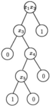
One way to solve the replication problem is to use con junctions of the primitive literals at the decision nodes. To illustrate this solution, consider the two term formula discussed above. Assume we use the conjunction x1 . x2 as the test at the root node. Now, the right branch leads to a positive leaf that corresponds to the examples that satisfy the first term. The left branch leads to a rep resentation of the second term (see Figure 2). We can represent this term by single attributes as before, but now the replication problem has disappeared. If, in ad dition, we have a feature for the second term, x3 · x4 · x5 , we obtain a decision with only two internal nodes.
But, how to define appropriate features while learning from examples? One approach is to determine them a priori as combinations of the primitive attributes of a fixed type and size [Breiman et a/., 1984, llivest, 1987]. A second approach is to discover them after learning a decision tree. This schema has been used by Quinlan to infer production rules from a decision tree [Quinlan, l987a]. Quinlan's method generates a production rule from each path in the decision tree, and then simplifies them by removing irrelevant conditions (attributes) in the rule.
There are two main differences between this approach and the FRINGE algorithm we define in the next sec tion. First, Quinlan's method is a simplification proce dure, so to find an accurate set of production rules the initial decision tree has to already contain all the rele vant patterns. In view of the replication problem, this may require a large tree and a large training sample. For FRINGE only some patterns have to be present in the initial tree, other patterns may surface later as the it eration proceeds. Second, Quinlan's method maintains rules for both classes when learning a single concept. This representation may not be as efficient as FRINGE's representation for concepts with a small DNF descrip tion.
5 Learning Features
The FRINGE learning algorithm uses the following iter ative schema to define appropriate features . The algo rithm begins with a set V of primitive attributes, and creates a decision tree for a set of examples, choosing its decision variables from the set V. Then, a find-feature procedure generates new features as Boolean combina tions of the variables that occur near the fringe of the tree. We describe this heuristic in more detail below. The set of new features is added to the variable set, the examples are reexpressed using this expanded set of vari ables, and the execution of the decision tree algorithm and the find-feature procedure is repeated. We will call a single execution of both processes an iteration. The iterative process terminates when no new features are added to the variable set, or a maximum number of variables is reached.
The find-feature heuristic was originally designed to discover relevant conjunctions of the target concept. To see this, observe that a decision tree defines an equivalent DNF expression. Each path from the root node to a positive leaf defines a term as follows: initially, set the term to the constant value 1; then, for each node in the path form the conjunction of the current term and the attribute at the node if the path proceeds to the right of the node, otherwise form the conjunction of the current term and the negation of this attribute.
The find-feature procedure defines a feature for each positive leaf as follows: initialize the feature the constant value 1, and consider the path oflength two from the leaf. Then, for each node on the path, form the conjunction of the current feature and the attribute at the the node if the path proceeds to the right, otherwise form the conjunction of the current feature and the negation of the attribute. A leaf node with distance less than two from the root does not define a feature. So, the find-feature heuristic simply defines features by applying the term formation rule to the fringe of the tree. For example, the find-feature heuristic applied to the decision tree in Figure 1 would produce the features: X4 · xs, x4 · x5 , x1 · x2 (one feature appears twice). They correspond to the positive leaf nodes taken from left to right.
In each iteration, the find-feature heuristic forms very simple combinations: namely, conjunctions of two liter als. The creation of longer terms, or more complex fea tures, occurs adaptively through the iterative process. Initially, the variable set contains only the attributes. After the k-th iteration, the variable set may contain features of size up to 2k. For example, after the second iteration, a feature is either a term of size up to 4, or a conjunction of two clauses, each of size 1 or 2. Negated features include clauses of size up to 4, and disjunctions of two terms of size 1 or 2. In the limit, the find-feature procedure has the capability of generating any Boolean function of the literals, since the negation and and oper ators are a complete set of Boolean operators .
Figure 3 illustrates the learning performance results for a single execution of FRINGE on a small random DNF ( dnf4, see section 6) and how it compares to a strategy where features are proposed at random. The random proposal heuristic works as follows . A feature is defined as the conjunction of two elements chosen at random from the current variable set. Moreover, the ran dom proposal heuristic adds in each iteration the same number of features as FRINGE did. So, both methods work with the same number of variables in each iteration.
The graph shows the change in percentage error and in size of the hypothesis generated by the two methods as the iteration proceeds. The error is measured on a sam ple drawn from the uniform distribution independently of the training sample. More details on the experimental design are given in section 6.
The shape of the error and size graphs for FRINGE, given in Figure 3, are typical. After the first few iter ations, a very accurate hypothesis is usually developed, and the remaining few steps are used to reduce the size of the representation by introducing more meaningful features. Eventually, the process ends because the find feature procedure cannot discover any new features, and any further iterations would produce the same hypothe SIS.
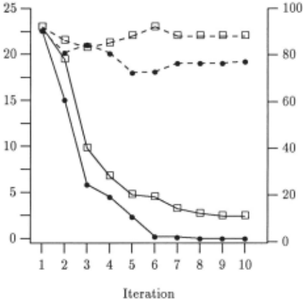
The random guess heuristic was not successful at all. The small fluctuations occur because by chance a few of the random combinations are significant.
Another interesting aspect of FRINGE's learning be havior is the form of the final hypothesis . In this exam ple, the test target concept has 10 terms in its small est DNF description and the final tree has 10 decision nodes . The decision variable at each node is exactly one conjunction in the original target concept. Hence, the complexity of the final decision tree is the same as the complexity of the smallest DNF representation for the concept. A similar behavior was observed for all DNF concepts, in the absence of noise, whose representation uses terms of approximately the same length. For DNF concepts with terms much longer than the average, the final hypothesis tends not to include them. However, the final hypothesis is still very accurate because the exam ples that only satisfy these long terms are rare when the examples are drawn from the uniform distribution.
To end this section, we discuss briefly how the find feature procedure can be generalized to accommodate continuous attributes, and multiple concepts. In a de cision tree a test for a continuous attribute defines a binary partition of the attribute range [Breiman et al., 1984] . Therefore, it can be thought of as a binary attribute, and the find feature procedure can be applied without modifications .
So far, only the positive leaves determine candidate features . A dual heuristic can be defined for CNF (Con junctive Normal Form) concepts by looking at the neg ative leaves, and by using disjunctions instead of con junctions. Moreover, a symmetric heuristic could be ob tained by applying the original find-feature procedure to the positive as well as to the negative leaves. This last heuristic can also be used in the multiple class case, by applying the feature formation rule to all leaves, regard less of their class label.
6 Experiments
The performance of a learning algorithm can be mea sured in terms of the classification accuracy on unseen instances from the target concept and in terms of the size of the final hypothesis. The goal of our experiments was to test how well the FRINGE algorithm does using these two criteria, and how well it compares with a decision tree algorithm with respect to the same criteria.
The algorithms were tested on five domains. They are: small random DNF, multiplexor, parity, majority and prob-disj . In addition, we tested the performance of the algorithms in the presence of random noise in both attributes and classification .
We present in Table 1 a concise description of the test functions by listing the total number of attributes, the number of terms, the average term length and the stan dard deviation from the average of the term length, in the smallest DNF description of the target concepts. The first four test functions ( dnfl - dnf4) are small random DNF functions [Pagallo and Haussler, 1988], mult11 is multiplexor on 11 attributes [Wilson, 1987], par4 and par5 are parity four and five attributes respectively [Pa gallo and Haussler, 1988], maj11 is majority out of 11 at tributes [Subutai and Tesauro, 1988], and prdsj is a short hand for prob-disj [Quinlan, 1987b] . For all test func tions except prdsj additional irrelevant attributes have been added.
We executed ten independent runs for each test func tion. The following design criteria for the sample sets were used for all domains except prdsj. For this domain we used the specifications given in [Quinlan , 1987b] to facilitate the comparison of results.
In each execution, the learning and testing tasks were performed on two sets of examples independently drawn from the uniform distribution . The learning set was ran domly partitioned into two subsets, training and pruning sets, using the ratios~ and~ [Breiman et a/., 1984] . The training set was used to generate a consistent hypothe sis. The pruning set was used to reduce the size of the hypothesis and (hopefully) to improve its classification performance on new instances of the target concept.
Let N be the number of attributes and I< be the num ber of literals needed to write down the smallest DNF description of the target concept. Let f be the percent age error that we wish to achieve during the testing task. The number of learning examples we used is given by the following formula:
| function id | attributes | terms | term avg. | length dev. |
|---|---|---|---|---|
| dnfl | 80 | 9 | 5.8 | 0.4 |
| dnf2 | 40 | 8 | 4.5 | 1.2 |
| dnf3 | 32 | 6 | 4.8 | 1.0 |
| dnf4 | 64 | 10 | 4.1 | 0.7 |
| multll | 32 | 8 | 4.0 | 0.0 |
| par4 | 16 | 8 | 4.0 | 0.0 |
| par5 | 32 | 5 | 5.0 | 0.0 |
| majll | 32 | 462 | 5.0 | 0.0 |
| prdsj | 10 | 3 | 3.0 | 0.0 |
This formula represents roughly the number of bits needed to express the target concept, times the inverse of the error. This is approximately the number of examples given in (Vapnik, 1982, Blumer et al., 1987] which would suffice for an ideal learning algorithm that only consid ers hypotheses that could be expressed with at most the number of bits needed for the target concept, and always produces a consistent hypothesis. Qualitatively, the for mula indicates that we require more training examples as the complexity of the concept increases or the error decreases. In our experiments we set f = 10%. We used 2000 examples to test classification performance.
Table 2 presents the results we obtained with the de cision tree algorithm and FRINGE for each target con cept. The table reports the average percentage error and the average tree size obtained over ten executions of the algorithms. The percentage error is the number of classi fication errors divided by the size of the test sample. The deviation of the actual results from the average error is within 7.3% for the decision tree algorithm and within 4.5% for FRINGE. The size of the tree is measured by the number of internal nodes.
FRINGE discovered the exact concept for dnfl, dnf3, dnf4, multill and par4. The small error for dn£2 and dnf3 results from the fact that one or two terms in the concepts are much longer than the average length. So, examples that satisfy only the longer terms are very rare, when the examples are drawn from the uniform distri bution. FRINGE did not include a description for the longer terms in the final hypothesis.
Majority and parity concepts, with a large number of inputs, are hard for decision trees. Majority is hard be cause there are a large number of terms in the smallest DNF representation of the concept, and hence there are a large number of terms is the smallest decision tree for the concept. Parity is hard when the examples are drawn from the uniform distribution because the attributes are not correlated with classification [Pagallo and Haussler, 1988]. FRINGE found an exact representation for par4, but it could not improve significantly on the poor per formance of the decision tree algorithm for parS. Both methods performed poorly on maj11.
| 7unction | avg.% error | avg. | tree size | |
|---|---|---|---|---|
| id | DTree | FRINGE | DTree | FRINGE |
| dntl | l:l.4 | 0.0 | 4~.7 | !:J.U |
| dnf2 | 10.4 | 0.5 | 52.4 | 7.6 |
| dnf3 | 7.4 | 0.3 | 45.4 | 6.1 |
| dnf4 | 24.9 | 0.0 | 93.9 | 10.0 |
| multll | 13.1 | 0.0 | 97.0 | 11.6 |
| par4 | 38.3 | 0.0 | 125.3 | 4.9 |
| par5 | 36.5 | 22.1 | 324.6 | 120.7 |
| majll | 18.7 | 15.4 | 132.6 | 72.6 |
| prdsj | 22.8 | 11.4 | 21.9 | 7.1 |
| noise | noise on attr avg.% error | noise on class avg. %error | ||
|---|---|---|---|---|
| level | DTree | FRINGE | DTree | FRINGE |
| 5% | 15.8 | 10:-J | 13.9 | 6.0 |
| 10% | 19.3 | 16.7 | 20.6 | 11.3 |
| 20% | 27.8 | 27.1 | 32.7 | 28.5 |
| 40% | 29.4 | 28.6 | 49.0 | 49.0 |
The results for prdsj are, to within experimental error, comparable to the results reported in [Quinlan, 1987b].
As an example of the sensitivity of the algorithms to noise we test them on the concept dn£2. Figure 3 summa rizes the performance results for the noise experiments with different levels of class and attribute noise. The av erage percentage error was taken over five execution of each algorithm. A noise level of n percent means that, with probability n percent the true value was flipped. For attribute noise, each attribute was corrupted inde pendently by the same noise level. In all experiments, the learning and testing sets were generated as for the noise free case, and the results are an average over five executions. The learning and testing sets were corrupted using the same type and level of noise. The table shows that FRINGE is more sensitive to attribute noise than class noise, as is the decision tree algorithm.
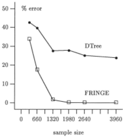
Another informative measure of the performance of a learning system is how the classification accuracy varies as a function of the number of learning instances. This variation is described by a learning curve. Figure 4 com pares the learning curves for the decision tree algorithm and FRINGE on dnf4. The percentage error is measured on an independent test set, and it is the average of five executions for each algorithm. FRINGE finds an exact representation for the target concept using a learning set of 1980 (or more) examples. A sample size of 1980 exam ples is the size of the learning set predicted by formula (1) for f = 10%.
7 Conclusions
In this paper we view the problem of learning from exam ples as the task of discovering an appropriate vocabulary for the problem at hand. We present a novel algorithm based on this approach. The algorithm uses a decision tree representation and it determines an appropriate vo cabulary through an iterative process. The method ac commodates target concepts that are described by dis crete as well as continuous attributes, and it can be used to learn multiple concepts simultaneously.
We also show empirically that this method compares very favorably on Boolean domains to an implementa tion of a standard decision tree algorithm for noise-free as well as noisy problems. Since the difficulties of the decision tree method arise from a representational limi tation, we expect that any reasonable implementation of this algorithm will give similar results.
Currently we are testing FRINGE on natural domains. So far, we have compared the methods on the mushroom [Schlimmer, 1986], hypothyroid [Quinlan, 1987b], and LED domains [Breiman et al., 1984], the latter with 10% attribute noise. The hypotheses generated by the deci sion tree method were already very accurate (less than 0.78% error) in the first two domains, and they were close to optimal (26.0% error, [Breiman et al., 1984]) in the LED domain. The hypotheses generated by FRINGE were more concise and at least as accurate.
Acknowledgments
I would like to thank David Haussler for helpful discus sions of the material presented here, and improvements to an earlier version of this paper. I also thank R. Bun tine, T. Dietterich, J . Schlimmer and P. Utgoff for helpful comments to a technical report that preceded this pa per. The support of the ONR grant N00014-86-K-0454 is gratefully acknowledged.
@inproceedings{ijcai1989p102,
  title     = {Learning DNF by Decision Trees},
  author    = {Pagallo, Giulia},
  booktitle = {Proceedings of the Eleventh International Joint Conference on
               Artificial Intelligence, {IJCAI-89}},
  publisher = {International Joint Conferences on Artificial Intelligence},
  editor    = {N. S. Sridharan},
  pages     = {639--643},
  year      = {1989},
  month     = {8},
  note      = {Machine Learning},
  url       = {https://ijcai.org/proceedings/1989/102},
}
TY - CPAPER TI - Learning DNF by Decision Trees AU - Pagallo, Giulia T2 - Proceedings of the Eleventh International Joint Conference on Artificial Intelligence, IJCAI-89 PB - International Joint Conferences on Artificial Intelligence PY - 1989 SP - 639 EP - 643 UR - https://ijcai.org/proceedings/1989/102 ER -Copied
Machine-readable versions of this paper, for tools and AI agents:





