Prioritized Defaults: Implementation by TMS and Application to Diagnosis

1 Introduction

Although the development of non-monotonic formalisms has been triggered by practical problems most work in this area has been devoted to the study of formal proper­ ties of non-monotonic inference. The technological value of non-monotonic formalisms is often ignored or ques­ tioned. We argue that non-monotonic logics can serve as intermediate formalisms in the development of ap­ plications for problems that require the generation and retraction of hypotheses. Good examples are diagnosis and configuration. Thus, we would decompose the de­ sign of an application into two steps:

1. Representation: First concentrate on the relevant representational decisions (e.g. what statements are encoded by hypotheses, defaults, priorities, coun­ terarguments etc.) without being concerned with technical details. The result of this step should be a comprehensive and implementation-independent so­ lution in terms of a non-monotonic formalism. Like a data-base scheme, it can be kept if the implemen­ tation is changed. This step also clarifies whether some properties of non-monotonic logics (e.g. multi­ ple extensions) are really problems or can be useful for applications.
2. Implementation: Different techniques can be used for implementi~~ a non-monotonic logic. If

they are already available the main task is to se­ lect techniques which are efficient for the special case under consideration. Thus, we can benefit from a lot of techniques (e.g. truth maintenance, dependency-directed backtracking) without being in trouble with technical details. Non-monotonic log­ ics serve as a specification for these techniques and show exactly how and in what circumstances they can be applied.

We illustrate this approach by developing a TMS­ based system for generating candidates for diagnosis. There are already several (A)TMS-based diagnosis sys­ tems (e.g. [de Kleer and Williams, 1987], [Struss and Dressler, 1989], [Dressler and Struss, 1990]). These works contain a lot of innovations how to do diagno­ sis. Unfortunately, parts of their results are hidden in the code and expressed in system-specific terms like jus­ tifications and labels.

Therefore, we consider an intermediate logic to do di­ agnosis (similar as [Poole, 1989]). We choose prioritized default logic [Brewka, 1989] where defaults are put into different levels of reliability. This allows to express pref­ erences such as 'adders are more reliable than multipli­ ers' or 'prefer correct models to fault models'. We discuss this topic in sections 2.2 and 2.3.

In a second step, we provide a general implementation oflevel-based default theories using TMS. Since they are equivalent to the special case of prioritized circumscrip­ tion implemented in [Baker and Ginsberg, 1989] we get an alternative method for handling prioritized circum­ scription. It does not need such notions as rebut and re­ fute. We just map every level of the default theory into a subnetwork of a TMS using the translation in [Junker and Konolige, 1990].

To verify our translation, we need some results on com­ ponents of TMS-networks. For this purpose, we split networks into independent components which can be la­ beled in isolation. Extensions of the complete network can be composed of extensions of the subnetworks. The precise results are presented in section 3.2. They are of their own interest because they enable a kind of divide­ and-conquer strategy for computing extensions. Thus, we have extended the work of Goodwin [Goodwin, 1987] who uses strongly connected components to guide the search in a particular labeling algorithm.

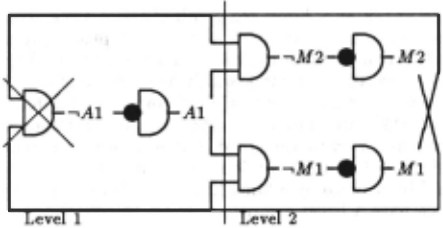
By linking the subnetworks of every level we obtain a TMS-network that reflects the level-structure of the default theory. Its extensions can be split in the same way as the preferred subtheories of the level-based de­ fault theory. This network is also obtained if we first ignore the levels and translate the defaults according to [Junker and Konolige, 1990]. Then we remove all justi­ fications leading from a higher level to a lower level (as illustrated in figure 1). It is difficult to imagine how a direct, ad-hoc approach to diagnosis could yield such a regular TMS-network.

2 From Diagnosis to Defaults

2.1 Prioritized Defaults

In this section, we introduce the non-monotoni$ formal­ ism which will be used to solve the diagnosis problem. We consider prioritized defaults [Brewka, 1989] which have been introduced by Gerd Brewka to extend the simple formalism of David Poole [Poole, 1988]. Unlike to Poole's Theorist, defaults can there be ordered into dif­ ferent levels L; of reliability. Defaults in L; have higher priority than defaults in Li+J: .

To formulate this precisely, consider a first-order lan­ guage £ including a special unsatisfiable constant 1... The first-order consequences of a subset X of £ are de­ fined as Th(X) := {q E £I X F q}.

Defaults are represented by a name q ( q is an atomic ground formula from£) and a premise q :::> <P (where <P is an arbitrary formula of£):

Definition 2.1 A level-based default theory 6. := (W, L) consists of a set W ~ £ of classical premises and a tupel L := (Lt, .. . , L~:) of disjoint levels L; containing atomic ground formulas from £ .

Preferred .subtheories of level-based default theories are defined recursively. A preferred subtheory of level i + 1 is obtained from a preferred subtheory of level i by adding elements of Li+l as long as consistency with W is ensured:

Definition 2.2 Let 6. = (W, (L1 , ... , L~:)) be a level­ based default theory. T is a preferred subtheory of level i iff

1. T = 0 if.i = 0

2. T is the union of a preferred subtheory T' of level i - 1 and a maximal subset of L; s. t. T U W ~ .l if iE{1, ... ,k}.

The preferred subtheories of 6. are the preferred subthe­ ories of level k.

We obtain Poole's Theorist if we consider only a sin­ gle level. Furthermore, if we already know a preferred subtheory T' of level i we could determine a subthe­ ory of the next level by supplying Theorist with T' as a set of premises and L;+l as a set of hypotheses. This view helps us to get a link to Reiter's default logic and from this to Doyle's TMS using the existing translation. Poole has shown that his simple hypotheses q correspond to prerequisite-free normal defaults ~ in Reiter's default logic. We define

Then Tis a preferred sub theory of level i+ 1 iff T consists of elements of levels and Th(T U W) is an extension of a default theory (DL,+t, W U T') a Ia Reiter which is supplied with a preferred subtheory T' of level i.

2.2 Diagnosis by Prioritized Defaults

In this section, we sketch how diagnosis problems can be formulated by level-based default theories. This in­ cludes statements for ranking different kinds of models (e.g. 'adders are more reliable than multipliers' or 'prefer correct models to fault models).

In the sequel, let 0 be a set of objects or components. Their normal and faulty behaviour is described by sev­ eral models 1 that exclude each other. The models of o E 0 are named by atomic formulas m; ( o) . For the sake of simplicity, we assume that every component has exactly k models .. A first-order theory W is used to de­ scribe the following facts :

• definition of the models (i .e. the behaviour of the single components)
• connections of pins or relationship between at­ tributes of different components
• values of the pins/attributes (including supplied in­ put values, as well as observed output values)
• exclusion of models (Vx.-.m;(x) V -.mj(x) fori "I j)
• completeness of models (Vx.mt(x) V ... V m~:(x))

We are interested in sets of hypotheses which explain the observed behaviour (i.e. the values of the output pins). A usual approach selects as many model as possi­ ble without violating consistency (models are selected by adding their names to the theory above) . This method treats every model in the same manner. However, we at least want to prefer normal models to fault models as in [Dressler and Struss, 1990]. A fault model should only be selected if a normal model is inconsistent with the current selection. Furthermore, it is useful to fo­ cus the diagnosis process to components that are more likely to fail. For example, cable connections often fail whereas TTL-circuits are reliable. We can easily ex­ press these preferences in a level-based default theory consisting of the first-order theory W and different lev­ els (L1 , ... , L;,Li+1 , ... ,L;+J:-d containing the names of models:

1 Models in the sense of model-based diagnosis.

• rank normal models of the components in 0 accord­ ing to their reliability and distribute them among the levels L1, .. . , L; .
• include the j-th fault model mj(o) of every component into Li+j-1·

Thus, we have also ranked the different fault models. Other rankings could be used for other approaches to diagnosis. Each preferred subtheory of this level-based default theory corresponds to a diagnosis candidate as defined in [Reiter, 1987] and [de Kleer and Williams, 1987]. To be more precisly, the negation of the correct models of the failing components are derived from the preferred subtheory. It is a maximal consistent subset of the set of models. Due to the preferences we do not obtain every candidate. Thus, diagnosis is focused to less robust components. A similar effect is achieved in [de Kleer, 1990] by preferring diagnoses with less faults.

2.3 Formulating Davis' Familiar Example

We illustrate our approach by the well-known adder­ multiplier circuit of Davis. It consists of two adders A1, A2 and three multipliers M1, M2, M3:

These components are connected as follows:

The correct models are described by a predicate ok and:

The supplied input and observed output values are:

In this example, we don't consider fault models. Let W be a first-order theory including the formulas above and further axioms for reasoning with equality and arithmetics 2 · Now, we built up a level-based default the­ ory Acirc = (W, L) where L := (L1, L2) consists of two levels. As a heuristc, we assume that adders are more reliable than multipliers:

Docirc has two preferred subtheories, namely:

Thus, only two of the four diagnosis candidates in [de Kleer and Williams, 1987] are obtained, namely

2 In practical systems, we realize equality and arithmetics using attached calls of lisp functions and simple propagation rules as in Steele's constraint-system.

{ -.ok(M1)} and { -.ok(M2), -.ok(M3)} . Thus, prefer­ ences have a similar effect as the fault probabilities in [de Kleer and Williams, 1987]: They focus the diagno­ sis process to candidates which are more likely to fail. Since we use a non-monotonic logic other candidates (e.g. {-.ok(A1)}) are obtained if additional observations (e.g. X = 6 and Y = 6) are added. Other approaches to diag­ nosis including fault models [Struss and Dressler, 1989] could be realized by adding these models to higher levels which have a lower priority.

3 Results for Doyle's TMS

Before we are able to map level-based default theories to TMS, we need some properties of TMS.

3.1 Relevant Properties of Doyle's TMS

In [Junker and Konolige, 1990], we developed a compact description of Doyle's TMS that is based on closures of operators. For a detailed discussion, we refer the reader to this work. We cite only the prerequisites for the theorems below: An operator apply : 2£ -+ 2£ mapping subsets of .C to subsets of .C is monotonic and compact iff

From this, we obtain a closure operation apply* as fol­ lows: apply*(X) is the minimal superset of X that is closed w.r.t. apply. Sometimes, apply depends only on a (relevant) part R of its input . In this case, it is suf­ ficient to iterate it on the relevant part to get (the rel­ evant part of) the closure. Hence, we take a restricted operator, which is expressed by the lambda-expression (~(X).apply(X) n R):

Lemma 3.1 Let apply : 2£ 1-+ 2£ be a monotonic and compact operator and R ~ .C s.t. apj:>ly(X) = apply(X n R) for all X ~ .C. Then apply*(0) n R = (~(X).apply(X) n R)*(0).

We obtain particular instances of such operators if we consider justification networks (N, J) of Doyle's TMS. N is a set ~of (arbitrary) nodes q from .C that are justi­ fied by non-monotonic justifications in J having the form (in(!), out(O) -+ q). Their inlists I and outlists 0 are both finite subsets of N. We obtain a monotonic and compact operator for applying justifications if we use an extra-index to check the outlist:

In contrast to the TMS-translation of unprioritized defaults, we supply justification networks with an input X ~ N, which is included in every TMS-extension:

Definition 3.1 Let v = (N, J) be a justification net­ work and X ~ N. T is an extension of v and X iff T = apply~ T(X). If v has no extension it is incoherent . '

If X = 0 we just say that T is an extension of v . The extra input X does not make the computation of exten­ sions more difficult . Its elements just get a fixed IN-label.

Now, we consider a set Q of nodes and denote their justifications by

If we are only interested in the part of the result of apply J,Y that is in Q we apply only justifications in fJ:

3.2 Clusters in TMS

In the sequel, we explore the structure ofTMS-networks. More precisely, we decompose a justification network into components which can be labeled in isolation. These components must not depend on the remaining network. A part of a justification network depends on another part if they are linked by a justification:

Definition 3.2 Let v = (N, J) be a justification net­ work, and C1 , C2 be two subsets of N. C2 depends on C1 if Jc 2 contains a justification (in( I), out(O)--+ c) s.t. (I u o) n c1 ::/: 0.

An independent component consists of nodes that have no justification depending on the rest of the net­ work.

Definition 3.3 Let v = (N, J) be a justification net­ work. Then C ~ N is an independent component of v iff C does not depend on N - C.

In the sequel, we explore properties of components. Nodes of an independent component C can only be de­ rived from nodes in this component .

Due to lemma 3.1 and equation 11, these properties can be extended to the closure of apply J,Y:

This allows to state one important property of inde­ pendent components: Every extension of the complete network can be split into an extension of the component and an extension of the remaining network and the first extension:

Theorem 3.2 Let v = (N, J) be a justification network, C be an independent component of v. T is an extension of v iff

Hence, we get an extension of T if we first find an extension of an independent component and then extend it further. In general, there is no guarantee that we find such an extension of an extension because the remaining network may be incoherent (due to odd loops). For level­ based default theories we will however obtain coherent subnetworks.

Networks which can be split into two independent components have an even nicer property: Their exten­ sions can be split completely. Hence, we can ignore the extensions of ( C, JC) if we determine an extension of (N- C, JN-c).

Theorem 3.3 Let v = (N, J) be a justification network that can be split into two independent components C and N- C. T is an extension of v iff

1. T n C is an extension of ( C, JC)

Due to these results we can take a divide-and-conquerapproach for computing extensions. We can compute ex­ tensions of independent subnetworks first, record them and then proceed to get extensions of dependent com­ ponents. Furthermore, we can combine extensions of different independent components without problems.

4 From Prioritized Defaults to TMS

In the next section, we consider the translation of a de­ fault theory a la Reiter to a TMS-network and modify it slightly to handle changing premise sets that are ob­ tained as results of lower levels.

4.1 Translating Default Logic to TMS

In [Junker and Konolige, 1990) we extracted two sets of formulas from Reiter's defaults. Let d = (D, W') be a default theory. We consider the set of consequents of defaults and the set of relevant formulas consisting of prerequisites and negated consistency assumptions of defaults:

Defaults and classical proofs are translated separately into justifications. Every default yields a non-monotonic justification:

Furthermore, we need all proofs of relevant formulas from premises W and consequents Cv. For this purpose, we define a set Mw (U, R) of monotonic justifications for a domain U ~ C, a rangeR~ C, and a theory W ~ C:

As pointed out in [Junker and Konolige, 1990), these minimal arguments for a goal q can be determined by consequence-finding algorithms based on linear-ordered resolution. The justifications in Mw(U, R) are sufficient to check for every element of R whether it can be derived from any subset of U.

In [Junker and Konolige, 1990], we have considered Mw·(Cv,Cv) for a default theory d = (D, W') . Here, we take a slightly changed encoding since we want to handle default theories with different premises. For this purpose, we split W' into a a fixed part W and a chang­ ing part X which is a subset of an upper bound C. Thus, we obtain a set of default theories forD, W, and C:

These default theories have a common TMS-network. Its non-monotonic justifications are NMD and its monotonic justifications are Mw(Cv UC,CD):

To regain the relevant part of an extension we supply the network with the additional premises X ~ C of the selected default theory:

Theorem 4.1 Let W and C be subsets of C and D be a set of defaults over C. Let X ~ C. There exists a bijective mapping of the set of extensions of (D, W U X) to the set of TMS-extensions of IID,w,c and X.

Using this network, we can handle default theories which differ in some part of their premise sets.

4.2 Mapping Levels to Clusters

Now, we are ready to map a level-based default theory (W, ( L1 , ... , L,.)) to TMS. We map every level to a TMS­ network getting the nodes of lower levels as input. It is important that the different subnetworks are disjoint (i.e. don't share any node). The translation profits from the results in [Junker and Konolige, 1990]: We relate every level to a default theory and map it to a TMS­ network using the translation in section 4.1. According to the results of section 3.2 we obtain the extensions of the complete TMS-network by a recursive characteriza-­ tion which is very similar to the definition of a preferred subtheory. Hence, it is not difficult to show that the extensions of this network are exactly the preferred sub­ theories of the level-based default theory.

Below, we elaborate this in detail. Let ~ = (W, ( L1 , ... , L,.)) be a level-based default theory. A pre­ ferred sub theory oflevel i is a subset of L~ := L1 U .. . UL; . As pointed out in section 2.1, we obtain for every level L; different default theories ~; := (DL;, W;) having a varying premise set W;. Such a set W; consists of W and a preferred subtheory of the next lower level which is a subset of L~_ 1 . Then we get the following result:

Theorem 4.2 Let ~ = (W, ( L1 , ·.. , L,.)) be a level­ based default theory. LetS; := {(DL;~ W U T') IT' is a preferred subtheory of level i- 1}. Then T is a preferred subtheory of level i itJT is an extension of a default the­ ory inS; .

In section 4.1, we extended the TMS-translation of default theories to capture changing premise sets. For level i, the changing part is CvL, containing all conse·-t quents of defaults of lower levels. Note that CvL · = L; ·and CvL, = Li sin~e the defaults in DL; have the simple form '7 for q E L;. Thus, we obtain the network 11; := IIDL . w L' · If we supply it with a preferred sub-·' , ·-1 theory of level i- 1 we get a preferred subtheory of level i as an extension of 11;.

Thus, we could get the preferred subtheories of the level-based default theory if we link the networks of its levels. Let 11; be equal to (N;, J;). First, we consider the networks for the levels 1 to i:

The complete network 11.0. is equal to II.O.,k ·

Now, we would like to apply the results of section 3.2 in order to relate the extensions of subnetworks to the preferred subtheories of a certain level. First, we have to identify independent components. Since every default is positive and occurs in exactly one level the sets N; of nodes are mutually disjoint. Hence, there is no justifica­ tion leading from N;-(Nl U .. . UN;_t) to N1 U ... UN;-1:

Lemma 4.3 Let~= (W, (L1, .·. , L,.)) be a level-based default theory. Then the set N1 U . . . U N;-1 of the nodes of II.O.,i-1 is an independent component of ll_o. ,;.

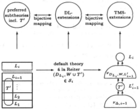
After getting all technical prerequisites, we are able to apply theorem 3.2 to the subnetworks of the level­ based default theory. Thus, we can prove the following theorem by induction on i using the theorems 4.2, 4.1, and 3.2 (cf. figure 2):

Theorem4.4 Let~= (W,(L1 , .. . ,L,.)) be a level­ based default theory. Then there exists a bijective map­ ping of the set of extensions of the subnetwork ll_o. ,; to the set of preferred subtheories of level i .

The mapping is indeed very simple: Just take the nodes of an extension that are in Li to obtain a preferred sub­ theory. In turn, we get the main result of this paper:

Theorem 4.5 (Main) Let~= (W,(L1 , ... ,L,.)) be a level-based default theory. Then there exists a bijective mapping of the set of extensions of the network ll_o. to the set of preferred subtheories of~-

Thus, we have translated a level-based default theory into a TMS-network. It reflects the level-structure of the default theory. It could also be obtained from the network of a level-free default theory by removing justi­ fications leading from a subnetwork of a higher level to a subnetwork of a lower level.

Our approach can also be applied to a restricted kind of prioritized circumscription which is obtained by adding unique names assumption and domain closure. Due to [Baker and Ginsberg, 1989], such a circumscrip­ tion theory can be mapped to a level-based default the­ ory, which is in turn translated to a TMS-network. For circumscription, goal-directed reasoning is required. To prove a goal q E C we need further justifications for proofs of q. After that, we can get rid of a large part of the network. According to theorem 3.2, we can focus our attention to the minimal independent component containing the goal q because the remaining subnetwork is coherent in this case.

4.3 Network for Davis' Familiar Example

Consider again the circuit example of section 2.3. In this section, we translate the default theory Llcirc into a TMS-network. The relevant first-order proofs can be extracted from the conflict sets, i.e. minimal sets of hy­ potheses that are inconsistent in conjunction with the premises. According to [de Kleer and Williams, 1987], we get two conflict sets:

We get the arguments for the relevant formulas -.ok(o) by applying the deduction theorem to the conflict sets.

Next, we consider the subnetworks for both levels. The first level contains only adders leading to two non­ monotonic justifications. v1 consists of

"\Ve don't get monotonic justifications in the first level because every conflict set contains some multiplier which belongs to a higher level. For the second level, we obtain a non-monotonic justification for each multiplier:

Additionally, v2 contains justifications for the negations of correct models of multipliers that are obtained from the conflicts of equation 20:

This network has two non-monotonic loops sharing -.ok(M1). To find labelings, we choose a label for this node and proceed with propagation. In general, we first consider networks for lower levels. Since the network lacks monotonic loops no groundedness check is neces­ sary as in [Junker and Konolige, 1990].

5 Conclusion

We pointed out how prioritized default theories [Brewka, 1989] can be used to obtain a TMS-based system for generating preferred diagnoses. To achieve this goal, we showed three results, which are of their own interest :

• Prioritized defaults allow to express preferences be­ tween models of behaviour in diagnosis from first principles. Thus, the diagnosis process can be fo­ cused to candidates that should be investigated first .
• Extensions of TMS-networks having independent components can be split into extensions of subnet­ works. Hence, divide-and-conquer methods may be used to compute extensions. An example for this is Goodwin's TMS-algorithm [Goodwin, 1987].
• Levels of defaults are mapped to TMS according to [Junker and Konolige, 1990] and then linked to­ gether using the result above. Thus, we get a TMS­ based prover for prioritized defaults which is an al­ ternative to Baker's and Ginsberg's prioritized cir­ cumscription prover [Baker and Ginsberg, 1989].

Priorities on general defaults have also been considered in [Brewka, 1989]. Our TMS-translation carries over to these defaults provided they don't share components. This condition ensures disjoint subnetworks.

An issue for future work is to see whether prioritized defaults can substitute fault probabilities [de Kleer and Williams, 1987], [de Kleer, 1990] in practical problems.

Acknowledgements

The different ideas presented in this paper arose from discussions with different persons. I would like to thank Prof. M. Richter, Kurt Konolige, Gerd Brewka, and Hans Voss. Peter Struss and Gerhard Friedrich gave helpful comments. This work has been supported by the Federal Ministry for Research and Technology within the joint project TAsso (Grant No. ITW8900A7) .