
High-Performance Aast Search Using Rapidly Growing Heuristics
Proceedings of the Twelfth International Joint Conference on Artificial Intelligence. Automated Reasoning. Pages 198-202.
© 1991 International Joint Conferences on Artificial Intelligence
Abstract
In high-performance A* searching to solve satisficing problems, there is a critical need to design heuristics which cause low time-complexity. In order for humans or machines to do this effectively, there must be an understanding of the domainindependent properties that such heuristics have . We show that, contrary to common belief, accuracy is not critical; the key issue is whether or not heuristic values are concentrated closely near a rapidly growing "central function." As an application, we show that, by "multiplying" heuristics, it is possible to reduce exponential average timecomplexity to polynomial. This is contrary to conclusions drawn from previous studies. Experimental and theoretical examples are given.
- [Bagchi and Sen, 1988] Bagchi, A., and Sen, A. Average- case analysis of heuristic search in tree-Like networks. In Search in Artificial Intelligence, ed. by L. Kanal and V. Kumar, New York: Springer-Verlag, pages 131-165, 1988.
- [Bramanti-Gregor and Davis, 1991] Bramanti-Gregor, A., and Davis, H.W. Learning admissible heuristics while solving problems. Proceedings of the 12th International Joint Conference on Artificial Intelligence, 1991. IJCAI
- [Chen, 1989] Chen, X. Generating and transforming heuristic functions to get desired properties. Master's Thesis, Wright State University, Department of Comput- er Science and Engineering, 1989.
- [Chenoweth, 1990] Chenoweth, S.V. An Analysis of the Asymptotic Performance of the A* Algorithm. Ph.D. Dissertation, Wright State University, Department of Computer Science and Engineering, 1990. See also: New approaches for understanding the asymptotic complexity of A* tree searching, by S.V. Chenoweth and H.W. Davis and The mathematical modeling of heuristics, by H.W. Davis and S.V. Chenoweth, to appear in Annals of Mathematics and Artificial Intelligence, Volume F. [Chenoweth and Davis, 1990]
- Chenwoeth, S.V., and Davis, H.W. Heuristics with folynomial growth patterns and the complexity of A* . n Methodologies for Intelligent Systems, Selected Papers, ed. by M.L. Emrich, et al, International Center for Application Technology, Knox- ville, TN, pages 49-62, 1990.
- [Christensen and Korf, 1986] Christensen, J ., and Korf, R.E. A united theory of heuristic evaluation functions and its application to learning. Proceedings of the AAAI, pages 148-152, 1986.
- [Garey and Johnson, 1979] Garey, M.R., and Johnson, D.S. Computers and Intractability, a Guide to the Theory of NP-Completeness. New York: W.H. Freeman and Company, 1979.
- [Gaschnig, 1979] Gaschnig, J. Performance Measurement and Analysis of Certain Search Algorithms. Ph.D. Dis- sertation, Carnegie-Mellon University, 1979.
- [Mostow and Prieditis, 1989] Mostow, J., and Prieditis, A.E. Discovering admissible heuristics by abstracting and optimizing: A transformational approach. Proceed- ings of the 11th International Joint Conference on Artifi- cial Intelligence, pp. 701-707, 1989. IJCAI
- [Pearl, 1984] Pearl, J. Heuristics: Intelligent Search Strategies for Computer Problem Solving. Reading, Massachusetts: Addison-Wesley Publishing Company, 1984.
- [Politowski, 1986] Politowski, G. On the Construction of Heuristic Functions. Ph.D. Thesis, U. C. Santa Cruz, 1986.
- [Rendell, 1983] Rendell , L. A new basis for state-space learning systems and a successful implementation. Arti- ficial Intelligence 20, pp. 369-392, 1983.
References were extracted automatically from the PDF and may contain errors.
Full text extracted automatically from the PDF; figures, tables and equations may differ. The PDF is the version of record.
1 Introduction
Two groups of studies, [Bagchi and Sen, 1988; Pearl, 1984, Chapter 7], have appeared in which heuristics are modeled as random variables (RV's); the model is used to determine what properties heuristics must have if A* is to have average polynomial, versus exponential, asymptotic time-complexity. The state space graph is assumed to be a uniform, b-ary tree, with start at the root, bi-directional arcs each of unit cost, and a single goal N units from start.1
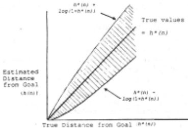
Let h*(n), h(n), respectively, return true and esti mated distance to goal from node n. The studies assume that the errors, h*(n) - h(n), suitably normalized, are independent and identically distributed RV's. We call this the "liD model" of heuristics. In the liD model, attaining average polynomial A* complexity is essentially equivalent to requiring that the values of h(n) be clustered near h*(n); the allowed deviation is a logarithmic function of h*(n) itself.2 See Figure 1.
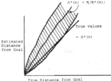
As a result of studies using the liD model, the impression has been given that high-performance A* search requires accurate heuristics. In this paper we describe a model which is more realistic than the liD model because it places no constraints on errors, or on h; we call it the "NC model." Conclusions from the NC model are not in agreement with those of the liD model: They predict polynomial A* complexity whenever the values of h(n) are logarithmically clustered near h*(n) + TJ(h*(n)), Henry W. Davis Wright State University Dept. of Computer Science Dayton, OH 45435
1Jn [Bagchi and Sen, 1988] the primary interest is in multiple goals. However, we discuss their results only for the single-goal problem, as that is our interest here. ·
2confer Theorems 3.1, 3.2 in [Bagchi and Sen, 1988] or Theorem 1 in [Pearl,1984, Chapter 7].
where TJ is an arbitrary, non-negative, non-decreasing function . See Figure 2. Heuristics whose values grow slower than distance to goal cause exponential complexity. See Figure 3. Ifwe think of clustering as a kind of"preci sion" and clustering near h* as "accuracy," then the differ ence is this: The liD model favors heuristics with loga rithmic accuracy and the NC model favors those which are rapidly growing and have logarithmic precision.
Sections 2, 3 state our results more precisely. Proofs are in an appendix. In Section 4 we apply the NC model to the phenomenon of "multiplying": That is, replacing a heuristic h with zh for some z ;:: 0. Studies with the liD model predict that multiplying is of no value in eliminating exponential complexity. The NC model, however, shows that multiplying can often change exponential A* complex ity to polynomial. Experimental and theoretical examples are given.
1.1 Motivation for the Mathematical Modeling of Heuristics
John Gaschnig's1979 dissertation [Gaschnig, 1979] gave the first thorough experimental results on the correla tion between the mathematical properties of heuristics and A* performance. His opening sentence states that the work is "based on the premise that in the future more of the subject matter of artificial intelligence (AI) research will be understood mathematically than at present." We agree with Gaschnig's view that establishing such founda tions is a challenging, long-term AI objective.
Gaschnig proposed a mathematical model to explain his data, but recognized that in large part it failed to do so [Gaschnig, 1979, Section 3.5.1]. Our motivation is based on the view that heuristics are central to AI, and that we cannot claim to understand them until we have mathemat ical models which explain experimental results obtained by using them.
Two other reasons for studying the mathematical properties of heuristics and how they affect search are as follows:
- Intractability results [Garey and Johnson, 1979] indi cate that many problems require a prohibitive amount of time to solve in the worst case. Compromises must be made. One type of compromise is to accept average polynomial time complexity. Heuristic search provides a mechanism for this, but we need a theory which tells us precisely when a heuristic provides such payoff.
- As our interest in increasingly hard problems grows, our need for good heuristics also grows. Several stud ies have been made about how humans and machines
may design such heuristics [Rendell, 1983; Pearl, 1984, Chapter 4; Christensen and Korf, 1986; Politowsk:i, 1986; Mostow and Prieditis, 1989; Bramanti-Gregor and Davis, 1991]. We believe that such research re quires a predictive mathematical model of heuristics. That is, there are domain-independent mathematical properties which a "good" heuristic has, and these must be understood if humans or machines are going to design them.
The A* algorithm is a sensible place to begin because (a) it is a very widely used heuristic search algorithm, and (b) although formally simple, it is not yet well understood how its performance relates to the mathematical properties of the heuristic it uses. Predictive models for A* should enable us to build better mathematical models for game tree searching, IDA*, AO*, and more sophisticated produc tion control strategies. One ultimate goal is that the search component in AI systems be based .more on scientif ic theory and less on ad hoc discoveries of the designer.
L2 Model Assumptions: Significance and Tradeoffs
A heuristic h is a function which returns a number when evaluated on a node n. What is the advantage in viewing h(n) as a RV? It is that we may view our complex ity conclusions as reflecting the aggregate properties of A* performance when A* is run over many problem instances. A possible disadvantage is that constraints made on the h(n) in order to make the mathematics tractable may not reflect the aggregate behavior of real heuristics. The re sulting conclusions about A* performance may be of limit ed use. This is a problem with the liD model. An appeal of the NC model is that no constraints are placed on the h(n).
The assumption that the state space graph is a b-ary tree is useful in providing potential for exponential explo sion. The assumption of a single goal is made here to simplify the mathematics. [Bagchi and Sen, 1988] have studied the multi-goal case in the liD model. This, plus the introduction of cycles, is interesting because it allows the possibility of compromising on solution quality when working on worst case intractable problems.!
2 Notation and Basic Relations
The graph, G, is an infinite uniform b-ary tree with bi-directional edges of unit cost. See Figure 4. The start node, nz, is at the root and a unique solution path n1, .. . ,nN+l leads to the goal, nN+l · which is N units away. The
l "Solution quality" refers to the extent to which the solution found is not optimal. It is not an issue when there is a single goal and the state space graph is a tree (as is assumed in this paper).
True Distance fro~ Goal
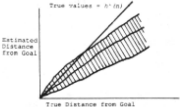
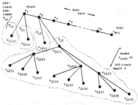
Figure 4. State space graph G with b = 3.
nodes nl> ... ,nN (excluding nN+l) are called on-track. Off track nodes are all other nodes, excluding nN+l and its descendants. The b-1 off-track children of ni form the roots ofthe off-track subtree Tui· 1 ~ u ~b-1 , 1 ~ i ~N.
Off-track nodes are denoted nuidv· where Tui denotes the off-track subtree containing nuidv· d ~ 1 indicates its depth, and v E {1, ... ,bd-1} references a particular node on level d within T ui·
We use the following symbolism:
| P[ ... ] | Probability of[ ... ]. |
| E[ ... ] | Expected value of[ ... ]. |
| k(n,m) | Cost or distance of shortest path from node n to node min G. |
| h*(n) g(n) | k(n,nN+l) k(nJ,n) |
| H (n,m) | Heuristic estimate of k(n,m) , a RV. We assume H(n,n)=O for all n E G. |
| h(n) | H(n,nN+J), a RV |
| f Z(N) Zui(N) | g+h Number of nodes expanded by A* when h*(nJ) = N Number of nodes on Tui expanded by A* when h*(n1) =N |
| exp(n) | Node nEG is expanded by A* |
| open(n) | Node n has been generated by A* |
| quidv | P[exp(nuidv) I open(nuidv)] , if P[open(nuidv)] > 0; otherwise it is zero. |
| max lf(njY: i+1 ~j ~ N+1}. max {j :f(n} =Ifti, i+l ~j~N+1}, a RV. | |
| If n = ni or nuidv , then nc = nljl(i) . Here 1 ~ i ~ N. | |
| The following formulas are used in the sequel: | |
| g(n;) = i-1, h*(n;) = N+1-i , | |
| (2.1) | { g(nuidvY = i+d-1, h*(nuidvY = d+N+1-i, k(nuidv ,ny = d+j-i, where 19,<j.g;+1, and d21. . |
3 Effects of Heuristic Growth and Clustering Patterns on A* Complexity
Let e(x) = tllog(l+t~3), where t · > 0, i = 1,2,3. Let 11 be a non-negative, non-decreasing function. For x :2: 0, define
(3.1) U(x) =X+ T)(x) + e(x) , L(x) =X+ TJ(X) - e(x).
We say his rapidly growing with logarithmic cluster if there exists~ E [0,1) such that
(3.2) For all off-track n = nuidv we have P[(h(n) :2: L(h*(n))) 1\ (h(noJ ~ U(h*(noJ) )] :2:1 - (!3/b)d.
Notice that the "central function," x + TJ(x), grows at least as fast as the diagonal, but is otherwise arbitrary. The intuitive meaning of the definition is that the h(n) are largely clustered within a logarithmic function of the central function h*(n) + T)(h*(n)). In more detail, off-track nodes have h-values mostly concentrated above a loga rithmic lower bound, and on-track nodes mostly below a logarithmic upper bound, with respect to this central func tion. For example, a special case occurs when each h(n) satisfies I h*(n) + TJ(h*(n)) - h(n) I ~ log(1+h*(n)), but is otherwise arbitrarily distributed. See Figure 2. Another example is shown in Figure 6 (which is discussed later); in the figure, h2 denotes the Manhattan distance for the 8Puzzle.
According to the theorem below, such clustering causes A* polynomial complexity on average, and also in the worst case if~ = 0 (which happens in Figures 2, 6).
Theorem ! (Logarithmic Cluster Complexity Theorem). If h is rapidly growing with logarithmic cluster then E[Z(N)] is polynomial inN; also, Z(N) is polynomial if~ = 0 in (3.2).
As an example, we ran A* on the graph of Figure 4 with N up to 20 and b = 2. The heuristic h had values as in Figure 2 (logarithmic cluster) with T)(x) = x2. Within these constraints h was designed to be as misleading as possible, returning the maximum allowed number on-track and the minimum allowed number off-track. A* expanded N nodes; i.e., it had linear complexity. The high-performance of A* using this heuristic is surprising because the traditional view, based on the liD model, is that good heuristics need to be accurate.
In contrast to Theorem 1, the theorem and corollary below show that slowly growing heuristics cause exponen tial complexity. The corollary says to expect exponential complexity if the maximum of h(n)~values eventually grows slower than does h* (n). This is shown in Figure 3. The theorem has a more delicate interpretation: If h(n) for open off-track nodes is likely to be growing slower than h*(n) eventually, then we may expect exponential complex ity.
Theorem 2 (Slowly Growing Heuristic Com plexity Theorem). Suppose there exists a differen tiable function w such that for some £ E (0,1),
lim w'(x) < 1 - £ ,
and for some a E(l,b], some N1 a positive integer, we have that node n off-track and h·(n) >N1 imply
P[h(n) ~ w(h·(n)) I open(n)] :2: alb whenever P[open(n)] > 0.
Then E[Z(N)] is exponential inN.
Corollary. Let w be as in Theorem 2. If there exists integer N 1>0 such that P[h(n) ~ w(h·(n))] · 1 for all n satisfying h·(n) > N 1· then E[Z(N)] is expo nential.
4 Multiplying Heuristics to Reduce A* Complexity
If h is a heuristic function one might hope to lower A* complexity by using, instead of h, the multiplied h~~ tic zh where z :2: 0 is a real number. We call z a multiplier. [G'aschmg, 1979] first demonstrated via compelling stat:is tical evidence that the use of multipliers with heuristics can substantially reduce A* complexity.! Two other attempts have been made to explain with a mathematical model the effects of multiplying. Both use the liD model. [Pearl, 1984, see especially pp. 206, 209] concludes that multiplying cannot turn exponential growth rate into sub exponential. [Bagchi and Sen, 1988, page 158] conclude that search with multiplied heuristics, "in its average performance, appears to enjoy no clear advantage over ordinary heuristic search. "2
The NC model provides a simple rationale for ex pecting multiplications to reduce exponential search complexity to sub-exponential in many cases; it also sug gests a good multiplier: Suppose the maximum values of a heuristic h are growing slower than h* but that overall the heuristic values show a logarithmic cluster around some "central function." Choose z > 0 such that the central function, multiplied by z, grows faster than the diagonal, if such is possible. According to Theorems 1 and 2, above, replacing h by zh reduces A* complexity from exponential to polynomial. We give below experimental and theoretical examples of this.
4.1 Example 1 (Experimental)
The 8-Puzzle [Pearl, 1984, Section 1.1.2] is a sliding block problem whose state space graph is only a first approximation to the tree state space graph of our model. While relatively large (181,440 nodes, maximum h*-value 30), it is finite, does not have a uniform branching factor, and contains cycles. However, most cycles are quite long, making the state space graph rather "tree-like"; search trees built by A* on 8-Puzzle problems have average branching factors close to 1.4. We would hope that, to a first approximation, our model is applicable to this domain.
1Gaschnig proposed a mathematical model to explain his data, but recognized that it had significant sh?rtcomings [Gaschnig, 1979, Sec tion 3.5.1). In particular, for large multipliers the model predicted increasing complexity, the reverse of his experimental results [Gasch nig, 1979, p. 112).
2-rhe problem with using the liD model to study multiplied heuristics is that multiplying an liD-model heuristic may throw it out of the liD model. An example of this is given in [Ch!lnoweth, 1~90, C~pte~ 5). This reference also contains a more detailed analysis than IS gtven here of the effects of multiplying heuristics.
We use as a heuristic for A* the Manhattan distance, h2: This is the sum over all tiles of the horizontal and vertical distance of the tile from its goal position. Figure 5 shows the observed values of h2 from a sample of 1998 randomly generated problems. From the maxh plot and Theorem 2 we expect exponential complexity when A* uses g + h2 as its evaluation function. Figure 7, taken from a sample of 605 randomly generated problems, shows that this indeed occurs (z = 1 curve: Notice that the ordinate has a logarithmic scale).
Consider the avgh curve of Figure 5 as a "central function" around which h2-values cluster. We multiply h2 by 4 so that 4·avgh increases at least as fast as the diago nal, a requirement of Theorem 1. Figure 6 shows the result, and also that the values of 4h2 are concentrated within a logarithmic envelope of 4·avgh. According to Theorem 1 we may expect polynomial complexity when A* uses g + 4h2. The pattern of data observed in Figure 7 corroborates this expectation. It turns out that increasing the multiplier above 4 causes relatively little improvement in A* performance.
4.2 Example 2 (Theoretical)
There are many theoretical examples of heuristics for which multiplication transforms A* complexity from exponential to polynomial. For instance, let R(x) = (x + log(1+x))/2, S(x) = x/2, and let each h(n) be distributed arbitrarily between S(h*(n)) and R(h*(n)), as is shown in Figure 8. By Theorem 2, A* search is exponential when using h. By Theorem 1, it is polynomial when using zh, for anyz?:: 2.
5 Conclusions
In high-performance A* searching to solve satisficing problems, there is a critical need to design heuristics which cause low time-complexity. In order for humans or ma chines to do this effectively, there must be an understand ing of the domain-independent properties that such heuris tics have. We have shown that, contrary to previous belief, accuracy is not critical; the key issue is whether or not True Distance from Goal heuristic values are concentrated closely near a rapidly growing "central function."
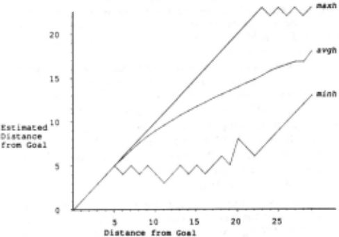
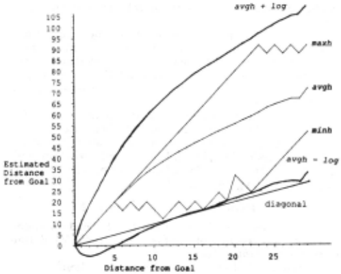
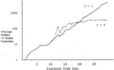
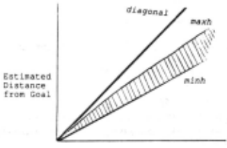
Figure 8. Values assumed by h in Example 2: maxh, minh are determined by the functions R, S described there. The state space graph is as in Figure 4.
· An open question is how much concentration, or clustering, is needed to assure polynomial time-complexity. We have shown that logarithmic clustering is adequate. Results reported in [Chenoweth, 1990; Chenoweth and Davis, 1990] show that the clustering can be polynomial when heuristic values grow fast enough. A necessary and sufficient condition for polynomial time-complexity is needed. ., ul · 1 · "
An application-related research ques~10.n 1s as follows: Admissibility and consistency of a heunsti~ can often be deduced by relating the heuristic to constramts of. t~e problem domain. See [Pearl, 1984, Chapter 4~ .. can simi lar considerations provide insight about heunstlc cluster ing patterns and growth rates?
As an application, we showed that, by ~ t1p ymg heuristics it is possible to reduce exponential average time-com~lexity to polynomial. This is contrary to the conclusion drawn from the traditional (liD) modeL. Expe~ imental and theoretical examples demonstratmg th1s result are given. . .
Appendix: Proofs for Theorems 1, 2
We make use of a function DN defined on nodes which are off-track or of the form n;., 15.ig{; We define DN(n) = k(n,nJ+h(nJ-h(n).
Lemma 3 is important because a node nuidv cannot be expanded if f(nuidJ > Ifti . This fact is used in the proof of Theorem 1.
The next lemmas are of a technical nature. Lemma 1· Assume y > 0. Then
(A.1)
x/log(N+x) <! y
for all x <! loga(2N) provided N ~ N 0 where e = aY, and N 0 <! 1 is chosen so large that
Take any N <! N 0 . By (A.2), loga(2N) 5. N. We consider two cases:
Case ill: loga(2N) 5. x 5. N. Then by (1 ),
y log(N+x) 5. loga(2N) , as x 5. N
5. x , by assumption on x,
which is (A.1).
Case {ID: x > N. Since x > N <!No , (A.2) implies
(2)
loga(2x) 5. x . Thus, by (1),
y log(N+x) < loga(2x) , since x > N
5, X, by (2),
again yielding (A.1). Q.E.D.
Lemma§.. Let e(x) = tllog(1 + 1~3), where ti > 0, i = 1,2,3. Let A. > 0, and suppose M is a positive integer. Then
(A.3) 2d/e(d+M) <!A. whenever
d <! loga(2M) , and
(A. 4 ) a = exp(l!A.ct 1 ts) ; where
{
c = log 3 I log 2 ; and where M satisfies
{
(A.S) M <!max( (2/t 2 )lfts, (V2)aA.cttlog 12, N1 ),
(A.6) where y <! N1 impliesloga(2y) 5. Y · Proof. First note that our choice of c in (A.5) gives c log(v) <! log(l+v) for all v <! 2, which is easily checked.
1When one relation involving RV's is derived from another using simple algebraic transformations, we omit stating the .. with probability 1 .. constraint.
(A.3) is true provided
(1) dl[c log(t:z{d+M}3)] <! A.t1 12
because of (A.5) and the first part of (A.6). But (1) is true provided dl{log t2 + t3log[d+Mll <! A.ct 12 , or (2) (log t2)/d + (t3log(d+M))/d 5. 21[A.ct1] . .
By Lemma 4 (withx=d, y=A.ct1t3, andNo=NJ),
[t3log(d+M)]Id 5, 1/[A.ctl]
provided (A.4) holds and M <! N 1. For such d the left side of (2) is 5. [log t2]1[log 0 (2M)] + 1/[A.ctl] 5, 2/[A.ctl] provided [log t2]1[loga(2M)] 5, 1/[A.ctl] ; that is,
(3)
which is included in (A.6). This proves (A.3). Q.E.D.
log 0 (2M) <! A.ct1log(t~ ,
Lemma 6. Let e be as in Lemma 5. Set A. = 3 and M .. N (= h*(n1)) in (A.4), (A.5), and (A.6). Assume there exist p E [0,1) such that for all off· track nodes nuidv we have P[exp(nuidv>l 5, (p!b)d whenever (A.4), (A.5), and (A.6) hold. Then E[Z(NJ] is polynomial in N. If P=O, then Z(N) is polynomial.
Proof.. Set M = N in the statement of Lemma 5. Let L(N) = loga(2N), where a is as in (A.4). Consider any N greater than the right side of (A.6). Then, for any off-track sub-tree T ui , we have
5. N + [2Nb bLrNJ] I [1-Pl ,
which is polynomial. If P=O, then, with probability 1, the left side of (1) may be replaced by Zu/N) and the summa tion on the right side involves only d < L(N). Thus, each Zui(N), and hence Z(N), is polynomial. Q.E.D.
Proof 2f Theorem !. We will prove the theorem by applying Lemma 6. To this end, let p be as in (3.2), and let n=nuidv be an arbitrary off-track node. Let (A.4), (A.5), (A.6) hold with M replaced by N, and A.= 3. We must show that P[exp(n)] 5. (p!b)d.
Applying (3.2) gives, with probability<! 1-(p!b)d, that DN(n) = k(n,nJ+h(nJ-h(n) 5, k(n,nJ+U(h*(nJ)-L(h*(n))
= TJ(h*(nJ)-TJ{h*(n))+e(h*(nJ)+e(h*(n)) :S 2e(h*(n)).
Thus P[DN(n) <! 3e(h*(n))] :S (p!b)d. As h*(n) :S d+N and e is an increasing function, we get P[DN(n) <! 3e(d+N)] 5. (Pfb)d. Now apply (A.3) of Lemma 5 to this to get that P[DN(n) <! 2d] 5. (p!b)d. By Lemma 3, n cannot be expanded if DN(n) < 2d. Thus P[exp(n)] 5. P[DN(n) <! 2d] 5, (p!b)d, as was to be shown. Q.E.D.
The next lemma is an extension to our environment of the formula for E[Z(N)] that occurs in [Pearl, 1984, Chapter 6]. For quidv definition, see Section 2.
Lemma 1.. Let Wuid be the number of nodes A* expands at level d of the off-track subtree T ui · Then
where a(d,d,v) · v and, in general, nu,i m,a(d,m,v) is the level m ancestor in T ui of nuidv , m = 1,2, ... , d.
Proof. As A* finds a solution, ni is expanded, so open(nuill) is certain. Consequently P[exp(nuill)] =quill· As Tui contains only one node at level1, quill is also the expected number of expanded nodes at levell. This proves the lemma when d = 1.
Assume the lemma is true for the d - 1 case. We must show it is true for the d case. Now, since open(nuidv> if and only if exp(nu,i,d-l,a(d,d-l,v)),
Then, in either case,
This establishes (A.8) for the inductive step, whence it is generally true. Now (A. 7) follows for the inductive step by applying (A.8) : E[wuid1 is simply the sum over all level d nodes of the probability that each is expanded. Q.E.D.
Proof of Theorem ~ and the Corollary. Let q = 1 - £. We first note that
(1) w(x) s; q(x-t) + t for some t <! 1 and all x ~ t . This is because for x sufficient ly large, say, x ~ t ~ 1, w(x) both lies below the diagonal and has slope< q. Thus, for all x ~ t, w(x) lies below the line through (t , t) whose slope is q , that is, (1) holds. Let (jl(x) = (1-q)2xf(l+q) and let No= max{N1+t,[(1+q)t-1]/q}. We first show that, if n = nutdv , N >No and d s; (jl(N-t), u and v are arbitrary, then
(2) P[exp(n) I open(nutdv)1 ~ alb whenever P[open{n)] > 0. For all such Nand d, N >No<! [(1+q)t -1] /q, so qN + N > (1+q)t -1 + N; that is,
= [(1+q)/{1-q)](jl(N-t) ~ [(1+q)/(1-q)]d.
Multiplying both sides by 1-q and separating N gives
(3) N > q(N+1-2t+d)-1+2t+d = (q[{N+d+1-t)-t]+t}+(d+t-1}
~ (w(N+d+1-t)} + (d+t-1} by (1),
= w(h*(nutdJ) + g(nutdJ · Notice that h*(nutdJ = N+d+1-t ~ (Nl+t)+d+1-t > N1. Thus, ifP[open(nutdv)] > 0 then
alb S P[h(n) S w(h*(n)) I open(n)] by our hypothesis
- = P[trn) :S w(h*(n)) + g(n) I open(n)]
- s; P[trn) < N I open(n)] , by (3)
- s; P[trn) < f(ncJ I open(n)] , since f(nN+l)=N
- S P[exp(n) I open(n)], which establishes (2).
To complete the proof of the theorem apply Lemma 7: E[Z(N)] ~ E[Zut<NJ], where u E (1, ... ,b-1},
~ [ a.<P(N-tJ] I <Xh , which is exponential inN. This proves Theorem 2.
The corollary follows from the theorem by noting that P[h(n) s; w(h*(n))] = 1 implies that P[(h(n) s; w(h*(n))) "open(n)] = P[open(n)] and so P[h(n) s; w(h*(n)) I open(n)] =1. Q.E.D.
@inproceedings{ijcai1991p30,
  title     = {High-Performance Aast Search Using Rapidly Growing Heuristics},
  author    = {Chenoweth, Stephen V. and Davis, Henry W.},
  booktitle = {Proceedings of the Twelfth International Joint Conference on
               Artificial Intelligence, {IJCAI-91}},
  publisher = {International Joint Conferences on Artificial Intelligence},
  editor    = {John Mylopoulos and Ray Reiter},
  pages     = {198--202},
  year      = {1991},
  month     = {8},
  note      = {Automated Reasoning},
  url       = {https://ijcai.org/proceedings/1991/30},
}
TY - CPAPER TI - High-Performance Aast Search Using Rapidly Growing Heuristics AU - Chenoweth, Stephen V. AU - Davis, Henry W. T2 - Proceedings of the Twelfth International Joint Conference on Artificial Intelligence, IJCAI-91 PB - International Joint Conferences on Artificial Intelligence PY - 1991 SP - 198 EP - 202 UR - https://ijcai.org/proceedings/1991/30 ER -Copied
Machine-readable versions of this paper, for tools and AI agents:





