
Learning Admissible Heuristics while Solving Problems
Proceedings of the Twelfth International Joint Conference on Artificial Intelligence. Automated Reasoning. Pages 184-190.
© 1991 International Joint Conferences on Artificial Intelligence
Abstract
A method is presented that causes A .. to return high quality solutions while solving a set of problems using a non-admissible heuristic. The heuristic guiding the search changes as new information is learned during the search, and it converges to an admissible heuristic which 'contains the insight' of the original nonadmissible one. After a finite number of problems, A .. returns only optimal solutions. Experiments on sliding tile problems suggest that learning occurs very fast. Beginning with hundreds of randomly generated problems and an overestimating heuristic, the system learned sufficiently fast that only the first problem was solved non-optimally. As an application we show how one may construct heuristics for finding high quality solutions at lower cost than those returned by A .. using available admissible heuristics.
- Davis et al., 1989)
- Davis H.W., Bramanti-Gregor A., and Chen X., Towards finding optimal solutions with non- admissible heuristics: a new technique, Proceedings of the 11th International Joint Conference on Artificial Intelligence, 303-308, 1989.
- Nilsson, 1980)
- Nilsson N .J., Principle of Artificial Intelligence, Tioga Publishing Co., Palo Alto, Ca., 1980.
- Politowski, 1986)
- Politowski G., On the Construction of Heuristic Functions, Ph.D. Thesis, University of California, Santa Barbara, 1986.
- Ratner et al ., 1986)
- Ratner D. and Warmuth M., Finding a shortest solution for the NxN extension of the 15-puzzle is intractable, Proceedings of the 5th National Conference on AI(1986) 16&-172.
- Bramanti-Gregor and Davis
References were extracted automatically from the PDF and may contain errors.
Full text extracted automatically from the PDF; figures, tables and equations may differ. The PDF is the version of record.
1 Introduction
A problem with A .. is that it often gives low quality solutions when its heuristic overestimates 1 · Optimal or near-optimal solutions are often desired and a strong underestimating heuristic is not always available. In [Davis et al., 1989] we describe how an admissible heuristic hM can be derived from a non-admissible heuristic h. The potential savings in node expansions when A .. uses g+hM as an evaluator (denoted A ·(hM)) is shown to be considerable' when compared to previously suggested methods that attempt to find optimal solutions with non-admissible heuristics.
In this paper we extend the definition of hM to an admissible heuristic which includes the 'collective insight' of one or more available heuristics. Using the hM concept, we describe a method whereby, while solving a set of problems, the quality of the solutions returned by A .. can be made to steadily improve. As more problems are solved, a dynamically changing approximation to hM, denoted rl!M, is learned. As it is learned, rlzM is also used to guide the search. We prove that, in a probabilistic sense, rhM converges to hM, causing A ·(rizM) to be admissible after a finite number of problems have been solved.
Variations of the learning technique are described.
1 A solution has 'high quality' when the ratio of its length to the optimal solution length is close to one.
These are chosen based on the amount of computation per problem the user wishes to invest in improving solution quality. In constant learning the overhead per problem is very low: a single relatively small computation. A user who is continuously using A .. in some domain may keep this type of learning active indefinitely. His system will evolve, at low cost, but slowly, towards the finding of optimal solutions. Quadratic learning requires more computation per problem than constant learning but riiM converges to hM after solving fewer problems.
In many applications high quality satisficing solutions are more desirable than optimal ones if they can be found with low time-overhead. We propose using quadratic learning to address this problem, by turning off the learning early so that the heuristic developed can be used before it evolves any further. This technique of turning off the learning early in the problem session is called here early learning. The purpose is to create a heuristic which (1) causes A .. to find high quality solutions, and (2) causes A .. to expand a relatively small number of nodes.
Experiments were performed in the 8-puzzle domain to get some empirical insight into the technique's effectiveness. We tested two available non-admissible heuristics, sometimes in combination with an admissible one. We used quadratic learning on samples of1998 and 605 randomly generated problems. The results of two groups of experiments are described in this paper. In one group we gauged the speed of learning. It was fast: The preponderance of information learned is acquired within eight randomly chosen problems. In all but the first problem, during which much of the learning occurs, A .. always returned optimal solutions.
In the second group of experiments we attempted to measure the effectiveness of using the early learning method to build heuristics. We combined non-admissible heuristics with an admissible one; our goal was to learn a composite heuristic which would cause A .. to return high quality solutions while expanding fewer nodes than when using the admissible heuristic alone. In ·one of the expe riments reported below, the learned heuristic returned solution quality within 6% of optimal while reducing by half the number of nodes expanded by A ·. In another experiment the system learned a heuristic which always returned optimal solutions at a 15% reduction in node expansion; however we cannot guarantee that the solutions returned will always be optimal. We conclude that the proposed method of building composite heuristics through learning shows promise of being useful.
2 Notation and Preliminaries
We use the following notation:
| R+ | Non-negative real numbers. |
| G | Locally finite directed graph with arc length bounded below by a positive number. |
| problem | An element (s,t)eGxG. sis viewed as the start and t as the goal. |
| k(m,n) | Length in G of minimum length path from m to n; oo if there is none. |
| h*(n) | k(n,t) where the goal t is implicit. |
| H(m,n) | heuristic estimate of k(m,n). Assume H(m,n) e R+ and H(n,n) = 0 for all n e G. |
| H(n,t); when t is implicit we write h(n). We think of t as a goal. | |
| g(n) | Shortest distance yet found by A • from start state ton. |
| A *(h 1 ), A *(h) | A • algorithm using g + h 1 as an evaluation function; when t is implicit, we write A *(h). |
| X | Number of nodes expanded by A • on some problem. |
| SQ | Solution quality: ratio of length of solution returned by A • to the optimal length. |
| admissible | Either h 5 h* or, equivalently, H 5 k. An algorithm is admissible if it returns optimal solutions when given solvable problems. |
An example used later is the 8-puzzle, a sliding tile problem (see, eg., [Pearl, 1984] or [Nilsson, 1980]). A common admissible heuristic for it is the 'Manhattan distance': H(m,n) denotes the sum over all tiles of the vertical and horizontal distance of each tile in m from its position in n. The problem of finding an optimal path connecting two 8-puzzle states is part of a family of NP-hard problems [Ratner et al ., 1986].
If His a heuristic, define for all x eR+
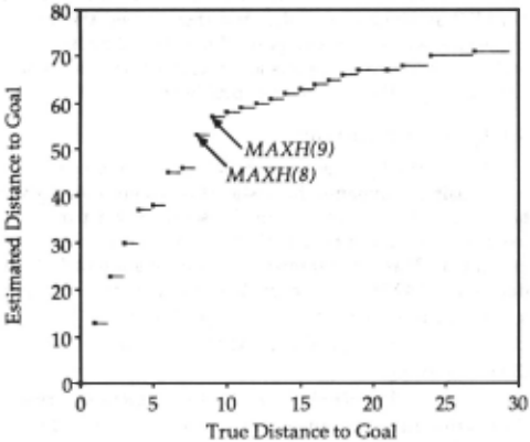
(2.1) MAXH(x) = max{H(m,n): (m,n) e GxG, k(m,n) 5 x). For example, a simple enhancement of the Manhattan distance is obtained by adding to it a 'sequence score' term (see [Nilsson, 1980, p. 85]). Denote the enhancement H3. MAXH3 is shown in Figure 2.1. In general, MAXH is a non decreasing function. If G is finite, then it is a step function whose value at any jump-point is the higher of the two alternatives.2
hM is defined in [Davis et al., 1989] and redefined here.
Let H be a heuristic estimate (admissible or not) and let hf(n) = H(n,t). For all n e G define (2.2) hfM(n) = min{x: hf(n) 5MAXH(x), x eR+}.
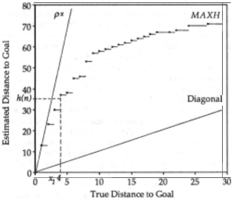
We write hM(n), instead of hfM(n), when context allows. Definition (2.2) and the reason why htM is admissible are best understood with a picture: In Figure 2.2 we let H, and its associated h, be the enhanced Manhattan distance, discussed above. Suppose, for example, hf(n) = 35. (2.2) says that, to find hfM(n) on the x axis, project horizontally to MAXH from 35 on they-axis and then vertically to the x axis. The resulting value, 4, is defined to be hfM(n). hfM(n) 5 h*(n) because, if h*(n) were less than 4, say x1, then there would be an x 1 < 4 with MAXH(x1) ~35, contrary to the way we obtain hfM(n). Thus htM is admissible.
2 If G is infinite, then the 'max' operator in (2.1) and the 'min' operator in (2.2), below, should be thought of as 'supremum' and 'infimum', respectively.
A note on the case when the H we start with is admissible: In this event MAXH never rises above the diagonal of Figure 2.2, whence, ht M ~ ht; ie., hM is at least as informed as h. This suggests a superiority of hM over h because more informed admissible heuristics cause less node expansion [Nilsson, 1980]. However, usually hM = h because it is common for MAXH( x) to lie on the diagonal when h is admissible. (For example, hM = h when h is the Manhattan distance.)
Finally, we wish to extend definition (2.2) to an admissible heuristic which 'captures the insight' of several given heuristic h1, ... ,hp (admissible or not). Define a heuristic ha, ... ,p)M· composed from h1, ... ,hp, as follows: Let htiM be given by (2.2) and let
(2.3) hta, ... ,p)M(n) = max(hf1M(n), ... , htpM(n)}.
ht(l, ... ,p)M is admissible and is at least as informed as htiM·
3 Learning and its Convergence
The critical question one asks when using hM in (2.2) is 'how do we compute MAXH?' In the learning technique, statistics are collected as A · runs enabling an approximation to MAXH, called rMAXH, to be built. This enables A· to use an approximation to hM, called rhM. rhM evolves over time. We discuss methods for learning rMAXH at different speeds, and then extend these ideas to the case when hM is composed from several heuristics. It is shown that, in a probabilistic sense, A ·(rhM) is admissible after solving a finite number of problems.
3.1 Quadratic learning.
LetS = {P1, P2, ... } be a set of problems to solve. A · is run on P1 using a dynamic heuristic rhM, where h is a given heuristic. rhM is dynamic in the sense that a parameter used in its computation changes as more nodes are expanded. This key parameter is an estimation of MAXH, denoted rMAXH. Whenever A· places a node non Open, n is assigned the heuristic value rhtM(n) where
(We write rhM instead of rhtM when context allows.) rMAXH is a non-decreasing function initialized to the zero function. It is updated as follows: suppose node n has just been selected from Open by A · and lets= n 0 , n1, ... , nj+1=n be the search tree path from s to n . Execute
Maintain rMAXH as a non-decreasing function The inner loop of (3.2) causes a possible increase in the recorded value of rMAXH(di). This may cause an increase in the recorded values of rMAXH(y) for many y > d; because rMAXH is to be maintained as non-decreasing.
As A · runs, (3.2) causes rMAXH to grow larger through a process of statistical sampling. When it is large enough to be useful, the lower part of (3.1) applies and rhM approximates hM. When not enough has been learned to use rMAXH, rhM behaves like h. Even though rMAXH alters over time, we do not reassign new heuristic values to previously generated nodes. When P1 is solved, the same procedure is now used to solve P2, except that rMAXH is initialized to the function developed during execution of P1, rather than to the zero function. The process of solving problems inS continues in this way.
Several aspects of (3.2) should be noted. It is possible that d; > k(n;,n) because the search tree path to n may not be optimal. Also H(n;,n) may not equal its maximum value for nodes separated by optimal paths of length k(n;,n). Both of these events contribute to make
(3.3) TMAXH(x) S MAXH(x) for all xt= R+
This, in turn, causes
(3.4) rntM(n) ~ htM(n) for all n, t € G,
when rMAXH has grown sufficiently large that the lower part of (3.1) is applicable. ·
The idea of the technique is that, as more is learned during problem solving, rMAXH increases to MAXH, rhM decreases to hM, and A ·( rhM) returns solutions of increasingly better quality while rhM converges to an admissible heuristic. The number of nodes expanded by A ·( rhM) on the other hand increases when compared with those expanded by A · using the unacceptable heuristic h. (This is because admissible heuristics, such as hM, force more breadth into the search.) One could turn off this learning process when the time-quality tradeoff is acceptable, and hold the current rMAXH fixed. The turn off point is determined by pragmatics because we cannot say with certainty how close the algorithm is to convergence at any time.3
Let X be the number of nodes expanded by A ·(rhM) in some problem. We call the procedure of (3.2) quadratic learning because the amount of time per problem directly spent in learning rMAXH is O(X2). To see this, notice that (3.2) is executed X + 1 times and, at each execution, rMAXH is updated at most X times (ie., j 5 X). The space needs of learning are small: an array whose size approximates the diameter of G to hold rMAXH when arc lengths are unit.
3.2 Reducing the time overhead of learning.
Linear learning differs from quadratic learning in that it takes fewer statistics per problem to learn rMAXH: When a node n is selected from Open we do not sample the search tree path to n, as in (3.2), but instead take a single sample:
(3.5) rMAXH(g(n)) r- max(rMAXH(g(n), H(s,n))
maintain rMAXH as a non-decreasing function
This is called 'linear' because the direct overhead of learning is O(X) per problem. It has the virtue that it may be kept active over a long period with substantially less time overhead than in the quadratic case.
The advantage of linear learning is accentuated by constant learning. In this only one statistic per problem is taken while learning rMAXH: Namely, (3.5) is performed only if n is a goal. The direct time overhead of learning on each problem is now a constant which is independent of the problem size. This kind of learning may be kept active indefinitely with only a very low time overhead. 4
3.3 Learning a composite of several heuristics.
Suppose, for example, we are given h1, h2 and we wish to form the approximation rii(1,2)M which should converge to ha,2JM· A direct way to proceed is as follows: In the gathering .of statistics (as described in (3.2) or (3.5)), both rMAXH;, i = 1, 2, are updated; use the rMAXHi so obtained to define mtiM by (3.1); finally, in analogy with (2.3), set
3 Several experiments with this 'early learning' technique are described in Section 4.3.
4 In practice, constant learning should be preceded by several runs using quadratic learning. Otherwise it may be a long time before rMAXH(x) is non-zero for low values of x. Learning credible values for these low x at an early time greatly enhances performance.
(3.6) mt(1,2)M(n) = max(mt1M(n), mt2M(n)}, for all nE G. In analogy with (3.4), one has, when both rMAXH i have grown sufficiently, that
mt(1,2)M(n) 2: hf(1,2)M(n) for all n,t E G. The technique extends to more than two heuristics in an obvious way.
If one of the h;, say h1, is already admissible, one could use a variant of (3.6) obtained by replacing rnt1M with hf1. As pointed out in Section 2, this substitution is equivalent to using hf1M when MAXH1 has its values on the 'diagonal'. Convergence of A · to an admissible algorithm is faster in this case. 5
3.4 A probabilistic Learning Theorem.
Will the learning described above eventually cause only optimal solutions to be found? The theorem below shows that, in a probabilistic sense, the answer is 'yes'. Proof is in the appendix.
Theorem 3.1 (Probabilistic Learning Theorem). Assume G is finite and that P1, P2, ... are randomly, and independently, generated problems from G.rG. Assume A·(mM) is using any one of the learning techniques described above. With probability 1, there exists i such that after P1, ... ,Pi. are solved we have: mtM = hfM for all t 0: G.
Hence, A·(mM) is admissible from some point on.
4. Experiments with Quadratic Learning
The effectiveness of learning may vary with the problem domain. To get some idea of what to expect, we conducted experiments in the 8-puzzle using the quadratic learning method. We used the Manhattan distance, h2, along with two non-admissible heuristics: h3, the enhanced Manhattan distance, and h4 . .Briefly, h4 adds to h2 weighted row-column and diagonal terms: the former counts the number of interchanged tile pairs which are in the proper row or column; the latter counts the number of tiles that are diagonally displaced and are blocked by in-place tiles. While h3 almost always overestimates and seldom finds optimal solutions, h4 normally under-estimates and usually, but not always, finds optimal solutions. 6
Our experiments were with rh3M, rlt4M, rh(2.JJM and rii(2,4JM· We had two sample sets: the first consisted of1998 randomly generated problems, and the second consisted of the initial605 problems of the first. We sometimes reor dered them to study how this affected experimental results.
4.1 Speed of Learning
We cannot know when the true MAXH has been learned because we do not know its value. However we can get an assesment of learning speed in the following way: Generate a large sample of random problems and record rMAXH when A·(rhM) is through solving the set of problems; now compare this rMAXH with the rMAXH which was learned at various 'snapshot points' during the problem solving session. This will show us how quickly the learning procedure acquired its final version of rMAXH.
5 If MAXH1 is not diagonal, then the heuristic converged to, while admissible, is not the same as ha,2JM and may be weaker. See discussion in Section 2.
6 h4 is a variation of a heuristic discovered semi automatically by Politowski [1986].
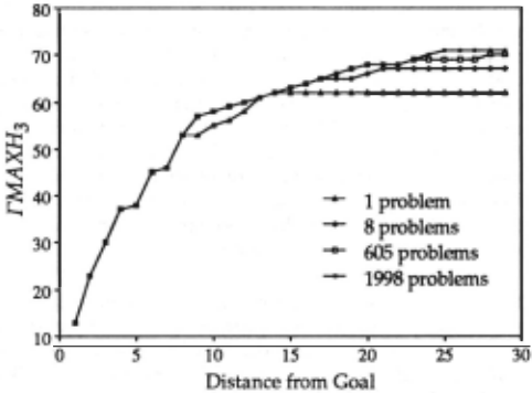
In the 8-puzzle, learning occurs quickly. For example, Figure 4.1 shows snapshots of how much A·(rn3M) learns while solving a set of 1998 randomly generated problems. After one problem rMAXH has been learned for distances 1 to 8 and after 8 problems through distance 17. Furthermore, at this point its knowledge of rMAXH for the remaining distances is within 6% of its final values. It acqui red no more knowledge after executing 1331 problems.
The pattern of Figure 4.1 was consistently observed: When the problems are randomly sorted, the vast amount of learning occurs within 8 problems. One could speed the learning process up by putting hard problems (ie., large start-goal distances) at the beginning and slow it down by putting easy ones first?
4.2 Solution Quality while Learning: Observation and Theory
We observed high solution quality while learning on randomly sorted problems sets: In our experiments A · returned an optimal solution in all but the first problem. This could not be guaranteed and surprised us. When the problems are arranged with the easy ones first, we observed that A · returned several non-optimal solutions.
In the proof of the learning theorem (see appendix) it is brought out that we may expect MAXH(.r) to be learned first for low values of x and then for higher values. This is the pattern shown in Figure 4.1 by the four successive snapshots of the knowledge acquired. Of course we don't know with certainty whether or not the true MAXH(x) is learned. When it is learned for all x 5 x 0 , say, then, according to the appendix, A·(rhM) returns optimal solutions for all problems whose start-goal distance is less or equal to x 0 · The observed behayior of A·(mM) suggests that the learned MAXH may, in fact, be correct.
7 In the experiments reported here the problems are randomly sorted and the first has start-goal distance of 19. This is considered a relatively easy problem because in the 8-puzzle the mean optimal distance between states is 22.
4.3 Early learning to build a composite heuristic
Suppose that, during a problem solving session with A ·( rhM), we stop the learning before all problems are solved. The heuristic which has evolved up to this turn-off point is said to have been acquired by early learning. Experiments were conducted to see how effectively early learning could be used to build a composite heuristic from two others. Our general finding is that, by early learning, the composite heuristic acquired is often one which produces high quality solutions at low cost. Cost is measured as number of nodes expanded per problem. We give two examples below.
Learning was allowed on only the first problem of the 605 sample set using A ·(m(2,4)M>· A .. was then run on the whole sample set using the heuristic learned in the first problem. See Table 4.1. Solution quality was within 6% of optimal and half as many nodes were expanded as were expanded by A ·(h2). The experiment shows that using early learning to add the insight of the non-admissible heuristic h4 to that of h2 creates a heuristic that reduces the cost of A · while making only limited compromises on solution quality. 8 On harder problems the cost reduction is higher (72%). Similar, but less spectacular results for A·(m(2,3)M) are also shown in Table 4.1.
In the second experiment A ·( rh(2,4)M) was allowed to learn on the first eight problems. Then, considering the entire sample set of 605 problems, we compared the performance of A .. using the heuristic learned in eight problems with the performances of A ·(h4) and A ·(h2). The result is shown in Table 4.2. A ·(m(2,4JM) produced perfect solution quality and expanded substantially fewer nodes then did the other algorithms: 15% fewer than A ·(h2) and 48% fewer than A ·(h~, with even better performance on the hard problems.9
Once the learning process is turned off, the use of rh(2,4)M requires only a little more time per node the'n the sum of that required to evaluate both h2 and h4; the extra time is for lookups into two tables of size bounded by the diameter of the graph, and a miximizing process. The resulting heuristic causes high quality solutions and relatively low node expansion count. In a general setting, the use of a composite heuristic like rh(2,4)M is justified if the computational time for evaluating both h2 and h4 is sufficiently low.
8 A · using h4 alone expands many more nodes than does A ·(h2)· See Table 4.3.
9 As h4 is usually optimistic it is tempting to combine h2 and h4 by forming the heuristic h24 = max(h2, h4). One could then compare the performance of A · using h24 with that of A·(ri1(2,4JM)· But it turns out that one always has h4 ~ h2 so h24 = h4. Thus there is no need to consider A ·(h24).
| avera~e eerformance | ||||||
|---|---|---|---|---|---|---|
| No. of | A •(m(2,3)M) | A •( rh(2,4)M) | ||||
| eroblems | SQ | X | %X2 | SQ | X | %X2 |
| easy (1-20) 187 | 1.02 | 170 | 96 | 1.03 | 152 | 86 |
| med (21-25) 346 | 1.05 | 645 | 79 | 1.07 | 496 | 61 |
| hard (26-29) 72 | 1.04 | 1236 | 51 | 1.07 | 679 | 28 |
| All (1-29) 605 | 1.04 | 569 | 70 | 1.06 | 411 | 51 |
Table 4.1 Performance comparison of A ·(rh(2,3)M) and A·(m(l,4)MJ with A·(h2). Early learning has occurred on one randomly chosen problem. Its start goal distance was 19. X denotes number of nodes expanded. SQ is solution quality (defined in Section 2) and is 1.00 for A·(h2).
| avera~e performance | |||||
|---|---|---|---|---|---|
| No. | of | A,.( rJit<2,4)M) | |||
| eroblems | SQ | X | %X2 | ~ | |
| easy (1-20) | 187 | 1.00 | 154 | 87 | 56 |
| med (21-25) | 346 | 1.00 | 704 | 86 | 54 |
| hard (26-29) | 72 | 1.00 | 2012 | 83 | 48 |
| All (1-29) | 605 | ( .. )1.00 | 690 | 85 | 52 |
Table 4.2 Performance comparison of A .. ( rsh(2,4)M) with A ,.(h 2 ) and A ,.(h4). Note (·): All solutions found were optimal but there is no guarantee that this will always happen. Early learning has pccurred on 8 problems.
avera~e eerformance
| No. of | A•(h2) | A,.(h3) | A•(h4) | |||
|---|---|---|---|---|---|---|
| eroblems | SQ | X2 | SQ | X3 | SQ | X4 |
| easy (1-20) 187 | 1.00 | 178 | 1.22 | 104 | 1.00 | 277 |
| med (21-25) 346 | 1.00 | 818 | 1.24 | 166 | 1.00 | 1312 |
| hard (26-29) 72 | 1.00 | 2427 | 120 | 208 | 1.00 | 4187 |
| All (1-29) 605 | 1.00 | 812 | 1.22 | 152 | (•)1.00 | 1334 |
Table 4.3. Performances of A ,.(h2), A ,.(h3) and A .. (h4) are given for comparison with previous data. h4 cau5es strong solution quality but poor time complexity. The opposite is true of h3. The text assumes that the solution quality of A ,.(h3) is unacceptable. Note (*): All but 10 solutions were optimal; 1.00 results from averaging to two decimal places.
5. Conclusion
It is possible to find optimal solutions with a non admissible heuristic h by letting A,. use g + hM as an evaluator, where hM is an admissible heuristic associated with h; hM contains much of the 'insight' that h has. There is a difficulty in calculating hM because it is based on an upper bound function for h which is hard to access.
We have described a technique for solving a set of problems using A .. (rhM), where rhM is a dynamically changing approximation of hM. As problems are solved, statistics are gathered enabling rl!M to evolve from h to hM. In the process, A,. returns solutions of increasingly better quality. We proved that, in a probabilistic sense, rl!M converges to hM, causing A .. (rl!M) to be admissible after a finite number of problems have been solved.
The above ideas extend to the case in which, instead of a single heuristic h, one starts with a finite set of heuristics, say ht, ... ,~~p. The admissible heuristic, hM, to which we now have convergence, is a composite of h1, ... ,hp (and contains their 'collective insight').
To gain some empirical understanding of this type of learning we performed experiments in the 8-puzzle domain using a variation of our technique called 'quadratic learning'. Learned information was acquired surprisingly quickly. The preponderance of information acquired in many hundreds of random problems was actually learned after solving only eight of them. Although we always started with an overestimating heuristic, the system learned so fast that all but the first problem were solved optimally.
In another experiment, we used 'early learning' to combine an admissible heuristic with a non-admissible one. The goal was to create a heuristic which caused A* to expand significantly fewer nodes than when it used the admissible heuristic alone; but nevertheless we wanted A* to yield high quality satisficing solutions. We were able to achieve this. In one case, for example, we obtained a reduction in node count of nearly half while only losing 6% in solution quality.
Our results show that it can be fruitful, while solving problems, to learn the statistical properties of the heuristic guiding the search. Knowledge of these properties may then be used to alter the heuristic itself, bestowing it with traits suitable to the application need. Moreover altering the heuristic can be done while the search is ongoing.
Appendix. Proof of Theorem 3.1
We give the argument for constant learning. This implies the linear and quadratic case because these learn at least as much in each problem as constant learning. For notational simplicity we do not consider the combined heuristic case of Section 3.3. The argument in that case is similar.
Let [a,b], [a,b) denote {x: xeR+, a ~x ~b) and {x: xeR+, a~ x <b) respectively. The theorem follows from the two lem mas below. We omit the proof of Lemma A.1, as it is clear. Lemma A.l. Suppose u > 0 and that at the end of some initial finite sequence of problems we have rMAXH(x)= MAXH(x) for all x e [0, u]. Then in any future problem (s,t) we have
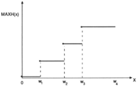
rhfM(n) = hfM(n) whenever neG and k(n,t) ~u. Lemma A.2. Let w1 < w2 < ... < wp be the discontinuity points of MAXH. Let W0=0 and let wp+l :?! wp be the length of the largest optimal path in G. Then given any je{0,1, ... ,p+1} there exists, with probability 1, some i such that after P1,. .. ,P; are solved by A*(rhM) we have for all future problems that (A.1) rMAXH(x) = MAXH(x) whenever xe [O,wjl
Proof: Figure A.1 illustrates the situation. We use induction on j . If j = 0, then (A.1) is clear. Assume (A.1) is true for j = k-1 . We must show it is true for j = k. Suppose the truth of (A.1) in the j = k-1 case occurs after P1, ... ,P; 1 have been solved.
If u > wk-1 and MAXH(u) = MAXH(wk_1) then (A.1) holds with Wj replaced by u; this is because both rMAXH and MAXH are non-decreasing, they agree at Wk-1, and rMAXH ~ MAXH. If k-1 = p and wp+l is not a discontinuity point (it is not in Figure A.l), then we are done. Assume that wk is a discontinuity point. Then, after solving Pt, ... ,P; 1 ,we have that for all future problems
(1) rMAXH(x) = MAXH(x) for all xe [O,wk)
We must show that, after solving more problems, the truth of (1) extends to wk.
Let (s,t)eGxG satisfy k(s,t) = wk and be such that H(s,t) is the largest number in {H(m,n): m, neG, k(m,n) = wk }. As the problems Pj are chosen randomly and independently from GxG, the probability of (s,t) never being chosen after Pt, ... ,P; 1 is zero. Thus, with probability 1, there is some i > i1 such that P; = (s,t). We shall show that after solving Pi we have (2) rMAXH(x) = MAXH(x) for all xe [O,wkl-
This will complete the induction and establish the lemma.
Lets= n 0 ,n1, ... ,nq = t be an optimal path for P;. In lemma A.1 set u = k(n1,t) to conclude that rhfM is optimistic on all the nodes n1, ... ,nq during the solution of P;, because of (1). After the first iteration of A*(rhfM), when n 0 is removed from Open, there will be a least r, 1 ~ r ~ q, such that n,e Open. For this node, g(n,)+rhf(n,) ~WJc, since n 0 , ··· ,nq is an optimal path. It follows that A*(rhfM), selects from Open, upon halting, an optimal goal for P;; that is, one whose g-value is wk. At this point, the constant learning procedure correctly updates rMAXH(wk) so that (2) holds. fl
@inproceedings{ijcai1991p28,
  title     = {Learning Admissible Heuristics while Solving Problems},
  author    = {Bramanti-Gregor, Anna and Davis, Henry W.},
  booktitle = {Proceedings of the Twelfth International Joint Conference on
               Artificial Intelligence, {IJCAI-91}},
  publisher = {International Joint Conferences on Artificial Intelligence},
  editor    = {John Mylopoulos and Ray Reiter},
  pages     = {184--190},
  year      = {1991},
  month     = {8},
  note      = {Automated Reasoning},
  url       = {https://ijcai.org/proceedings/1991/28},
}
TY - CPAPER TI - Learning Admissible Heuristics while Solving Problems AU - Bramanti-Gregor, Anna AU - Davis, Henry W. T2 - Proceedings of the Twelfth International Joint Conference on Artificial Intelligence, IJCAI-91 PB - International Joint Conferences on Artificial Intelligence PY - 1991 SP - 184 EP - 190 UR - https://ijcai.org/proceedings/1991/28 ER -Copied
Machine-readable versions of this paper, for tools and AI agents:





