
Qualitative Model Evolution
Proceedings of the Twelfth International Joint Conference on Artificial Intelligence. Vision. Pages 1311-1315.
© 1991 International Joint Conferences on Artificial Intelligence
Abstract
A pnetic aJsorithm is Ulled for JeanJiDs qualitative models b-I on the QSIM fOI'IIIalism. Hieran:hica1 :reprmentation eaables fonualion of "IIUbmodela" relevant for indudion of domain exp).anaQon. I>miDs the eean:h for better oocliDs of the c:audicWes, in puaiJel with the eean:h for better aoluuooa, the sise and shape -of candidate aolutiooa are dynamicaDy creaied. OpUmizaUon is baaed on the maximization of the number of examples covered by a candidate .110lution combined with the minimization of the number of 001111trainta Ulled in the aolution. The :result of J.eanUus is a lid. of models of difl'erent ..-=ific:ity that ezplain all pven examples. An experiment; in JeanJiDs a qualitative model of the COIIIltlded container BYBtem {UTUBE} is deacribed in detail. Several aolutiooa, equivalent to the OJ:isina1 model, were discovered.
- [Bratko et a./., 1991] Bratko, I., Muggleton, S. and Var!!ek, A. Learning qualitative models of dynamic systems, Inductive Logic Progra.mming ILP-91, Viana de Castelo, Portugal, 1991; also in: AI in Mathematics, Glasgow, 1991. 1316 Late Addition [Coiera, 1989] Coiera, E. Generating qualitative models from example behaviors, DCS Report No. 8901, School of Electrical Engineering and Computer Science, University of New South Wales, Sydney, Australia, 1989.
- Cramer, 1985)
- Cramer, N. L. A representation for the adaptive generation of simple sequential programs, Proceeding' of a.n lnterna.tiona.l Conference on Genetic Algorithm& a.nd Their Applica.tion1, pp. 183-187, 1985.
- Falkenheimer and Michalski, 1986) Falkenheimer, B .C. and Michalski, R.S. Integrating Quantitative and Qualitative Discovery: The ABACUS System, Ma.chine Lea.rning, Vol. 1, pp. 367-401, 1986.
- Feigenbaum, 1977)
- Feigenbaum, E. A. The Art of Artificial Intelligence 1: Themes and Case Studies of Knowledge Engineering. Pub. no. STAN-CS-77-621, Stanford University, Department of Computer Science, Stanford, California, 1977.
- Frantz, 1972)
- Frantz, D.R. Non-linearities in genetic adaptive search, Doctoral dissertation, University of Michigan, Dissertation Abstracts lntemational, 33 (11), 5240B-5241B, 1972.
- Goldberg and Lingle, 1985)
- Goldberg, D.E . and Lingle, R. Alleles, loci, and the traveling salesman problem, Proc. Int. Conf. on Genetic Algorithm& a.nd their Applica.tion&, pp. 154 - 159, 1985.
- Goldberg and Richardson, 1987)
- Goldberg, D .E. and Richardson, J. Genetic algorithms with sharing for multimodal function optimization, Genetic algorithms and their applications: Proceeding& of the Second lnterna.tiona.l Conference on Genetic Algorithm,, pp. 41-49, 1987.
- Goldberg, 1989)
- Goldberg, D.E. Genetic Algorithms in Search, Optimization, and Machine Learning, Addison-Wesley, 1989.
- Holland, 1975)
- Holland, J.H. Adaptation in natural and artificial systems, Ann Arbor: The University of Michigan Press, 1975.
- [Koza, 1989] Koza, J.R. Hierarchical Genetic Algorithms Operating on Populations of Computer Programs, Proc. 11th IJCAI, Detroit, Michigan, Aug. 1989, pp. 768-774, 1989. IJCAI
- Kuipers, 1986)
- Kuipers, B.J. Qualitative simulation, Artificia.l Intelligence, Vol. 29, pp. 289-338, 1986.
- Muggleton and Feng, 1990)
- Muggleton, S.H. and Feng, C. Efficient induction of logic programs, Proc. Fir1t Conf. on Algorithmic Lea.rning Theory, Tokyo, Sept . 1990.
- [Papadimitriou and Steiglitz, 1982] Papadimitriou, C.H. and Steiglitz, K. Combinatorial Optimization: Algorithms and Complexity, Prentice-Hall, Englewood Cliffs, NJ, 1982
References were extracted automatically from the PDF and may contain errors.
Full text extracted automatically from the PDF; figures, tables and equations may differ. The PDF is the version of record.
1 Introduction
Qualitative models successfully provide domain knowledge for many qualita~ive reasoning tasks. It is also recognized [Feigenbaum, 1977] that it is very difficult for a domain expert to articulate his "know how" into "say-how". Often, a domain Jllodel is not even known. One way to avoid this knowledge acquisition bottleneck is to provide a number of examples, from which a qualitative model of the domain can be automatically induced by means of machine learning techniques. ,
A method for learning qualitative models of dynamic systems from examples using g~netic algorithms is presented. This approach has been named Qualitative Model Evolution (QME). The problem, also known as system identification, is defined as follows: GIVEN examples and counter-examples of the system behavior, FIND a model that explains these examples. In this paper quantitative (i.e. numerical or differential equation) models are not considered. We are interested in qualitative models, where quantities are typically represented by a small set of qualitative values. Among several alternatives the QSIM formalism [Kuipers,
1986] was chosen for the representation of qualitative models because of its firm mathematical basis.
Learning is considered to be an instance of a combinatorial optimization problem [Papadimitriou and Steiglitz, 1982], i.e. a pair (F, c), where F is a finite or countably infinite set of feasible solutions and c: F -+ R is a cost function. The task is to find an f E F, such that Vy E F: c(f) ~ c(y). In our case, F is the set of all possible QSIM models in the given problem domain and c(f) is the number of examples correctly classified by the model f plus a bonus that decreases with the size of f. Genetic algorithms provide a robust framework for · performing such an optimization using Darwinian principles of reproduction and "the survival of the fittest".
Some work has been done on the automatic discovery of quantitative models but very little on the discovery of qualitative models of dynamic systems from examples. A brief description of some of the related approaches follows.
ABACUS [Falkenheimer, 1986] attempts to discover the best quantitative equation that describes a given set of numeric data in terms of addition, subtraction, multiplication and division.
GENMODEL [Coiera, 1989] creates the most specific generalization (expressed in the QSIM formalism) of examples. It initially generates the set of all constraints consistent with the first given example and then iteratively eliminates constraints that are inconsistent with the rest of the examples.
Bratko et al. [1991] use GOLEM [Muggleton and Feng, 1990] in a logic-based approach to find hypothesis H, given background knowledge B (the QSIM theory) and examples E, such that B A H f- E. An advantage of this approach is that GOLEM can introduce new variables into the model.
In Section 2 the QSIM formalism will be briefly described. The connected container system will be presented in Section 3. Section 4 introduces genetic algorithms and Section 5 describes our genetic algorithm that operates on populations of QSIM-based models. Experiments and the results obtained are described in Section 6.
A physical system is characterized by a set of physical parameters, which are continuously differentiable real valued functions of time. In QSIM, each of these parameters is represented by a function symbol. Furthermore, the domain of each parameter has to be specified in the form of a (small) totally ordered set of symbolic values, referred to as landmarks.
The current value of a parameter is stated in terms of its landmarks and the direction of change. The direction of change can be inc (increasing), std (steady), or dec (decreasing). If a parameter Pis equal to a and is increasing, this is written as P: a I inc. If, on the other hand, P is between a and b and is increasing this can be stated as P: a ... b I inc. Each physical system state is represented by a list of values for all parameters in the system.
A QSIM model is a set of qualitative differential equations, where relations among different parameters are expressed as constraints, such as monotonicity and derivative. A list of corresponding values can be used to specify particular points of a relation. The repertoire of QSIM consists of six types of constraints:
In the original Kuipers' paper legal ranges of parameter values are not treated in terms of constraints but are part of operating region definitions. In order to simplify our approach, a uniform representation is used by introducing one additional constraint:
Consider the two connected containers in Figure 1. The two containers A and B are connected with a pipe and filled with liquid to the non-negative levels La and Lb, respectively. Let Fab be the flow from A to B. This flow depends on the level difference Dab:
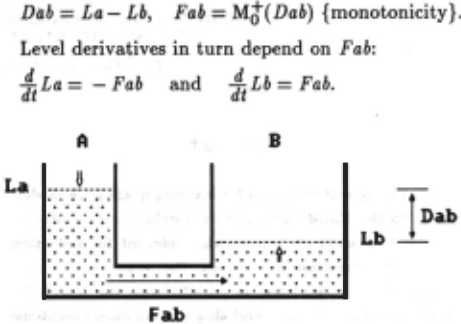
Let us formulate this in QSIM. There are five function symbols: {La, Lb, Dab, Fab, Fba}. In our example, appropriate landmarks for the five variables are: La: { -oo, 0, laO, oo }, Lb: { -oo, 0, lbO, oo }, Dab: { -oo, 0, dO, oo }, Fab: { -oo, 0, fO, oo} and Fba: {-oo, -fO, 0, oo}. We also have seven constraints that govern behavior.
Complete model:
Simplified model:
| RANGE(La,O ..• oo/ dec .• .inc) | RANGE(La,O •.. oo/ dec .. .inc) |
| RANGE(Lb,O ... oo/ dec .. .inc) | RANGE(Lb,O ••. oofdec .. .inc) |
| ADD(Dab,Lb,La,[( dO,lbO,laO)]) | ADD(Fab, Lb, La, [ ]) |
| MO_PLUS(Dab,Fab,[( dO,fO)]) MINUS(Fab, Fba, [(fO,-fO)]) | MINUS(Fab, Fba, [ ]) |
| DERIV(La, Fba) | DERIV(La, Fba) |
| DERIV(Lb, Fab) | DERIV(Lb, Fab) |
A simplified version of a model was used in the experiments in order to reduce the complexity. During the generation of training examples the model decides whether the state is legal or not. We have discarded the corresponding values and the (somewhat redundant) parameter Dab, together with the monotonicity constraint.
4 Genetic Algorithms
Genetic algorithms (GA) can be viewed as a general purpose search method, an optimization method, or a learning mechanism, based loosely on Darwinian principles of biological evolution: reproduction and "the survival of the fittest" together with genetic recombination [Holland, 1975; Goldberg, 1989].
GAs maintain a set of carulitltde sol·tions called a pop·lation. Candidate solutions are usually represented as binary strings of fixed length (called chromosomes). Given a (random) initial population GAs operate in cycles called generations:
- Each member of the population is evaluated using a fitness f-action. Evaluations can be normalized, scaled or left unchanged.
- The population undergoes reprod·ction in a number of iterations:
- genetic operators, such as crossover and mutation, are applied to parents to produce offspring.
- one or more parents are chosen stohastically, but strings with a higher . value of fitness function have higher probability of contributing an offspring;
- The offspring are inserted into the population. In some versions, the entire population is replaced in each cycle, while in others only a subset of the population is replaced.
The crossover operator produces two offspring (new candidate solutions) by recombining the information from two parents, whereas the mutation operator prevents irreversible loss of certain patterns by introducing small random changes into chromosomes. It has been proved [Holland, 1975] that mutation plays a decidedly secondary role in the operation of GAs.
A number of parameters can influence the algorithm, e.g. the size of the population, the size of the subpopulation replaced in each cycle, the probability of applying individual genetic operators, etc.
Superficially, it seems that GAs only process individual strings present in the population, but, in fact, they implicitly process large amounts of similarity templates or schemata representing numerous similar individuals not actually present in the current population. This leads to the key-stone of genetic algorithm approach: highly fit, short schemata are propagated through generations, giving exponentially increasing number of samples to the best schema observed in the population (although the number of individuals in the population is constant).
The effectiveness of a GA depends heavily on the chosen representation. Substantial effort has been focused on this problem: how do we know that the schemata contained in a given coding will lead to the desired improvement? For this reason, operators that change the coding in a search for better ones have been devised [Frantz, 1972; Holland, 1975; Goldberg and Lingle, 1985].
5 Qualitative Model Evolution
Our goal is to find a QSIM-based model that explains all given positive and negative examples. Positive examples represent legal states of a physical system and negative examples represent its illegal states. Two simplifying conditions were assumed in our experiments:
- All relevant physical parameters and landmark values must be known in advance.
- Only models with empty lists of corresponding values are considered (except for the implicit pair (0, 0) in Mri and M0 constraints).
Our GA operates on a population of QSIM-based models. Since the length of the solution is not known in advance, candidate models should vary in size. Furthermore, the coding of models should enable meaningful schemata (building blocks) to emerge. For this purpose the usual string-based representation seems unnatural and limited. We have used a richer structure: 6inarr trees [Cramer, 1985; Koza, 1989], where the leaves are QSIM constraints and branching points establish the hierarchical structure. This coding is position-independent since the model represented by such a tree consists of all constraints that occur in the tree.
The initial population consists of randomly created trees with uniform distribution of the number of leaves within the interval [1, Lmaxl· The size of the subtrees is also (recursively) determined randomly. However, later during the search reproduction may yield trees with more than Lmax leaves.
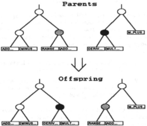
For our purpose genetic operators (crossover and mutation) had to be redefined in order to work on binary trees [Cramer, 1985; Koza, 1989]. C1'061!0ver operates on two parental trees in the manner illustrated in Figure 2. First, a node is selected uniformly at random in each parent and then the subtrees below the selected crossover points are exchanged (including crossover points), producing two offspring. Mutation operates on a single parental tree. First, a node in the parent tree is selected uniformly at random. Second, the subtree below the selected node is erased {including the selected point) and replaced by a randomly generated (sub )tree.
The learning process is considered to be a combinatorial optimization task based on the maximization of the number of examples covered by the candidate solution and on the minimization of the size of the candidate solution. The fitness value is calculated in three steps:
- raw fitness is determined,
- raw fitness is shared among similar individuals,
- shared fitness is scaled.
Step 1:
Let EP be the number of positive examples, En the number of negative examples, Cp(T) the number of positive examples covered by a tree T (i.e. consistent with the model represented by T), and Cn(T) the number of negative examples covered by T (i.e. recognized as illegal states). Furthermore, let L(T) denote the size of a model represented by T. The raw fitness primarily reflects the model's ability to cover training examples since the size of the model affects fitness value only when the model covers all training examples:
The shares of covered positive and negative examples are normalized to equalize their influence. If a candidate solution covers all training examples it receives a nonnegative bonus B that decreases with the size of the solution. K is used to scale the contribution of the model size to the fitness value with respect to the contribution of training examples. Throughout our experiments Llim = 2 · Lmax and K = 0.2 was used. These values were determined experimentally.
Step 2:
To prevent early convergence of the individuals, and to permit the formation of subpopulations (species) of individuals with common characteristics that exploit different subsets of the domain (niches), raw fitness is shared among similar individuals [Goldberg and Richardson, 1987].
The similarity function is defined for any two models to be the number of examples in which both models agree (they both either accept or reject the example). The degree of sharing S(T) for a tree T is then determined by summing up the similarity function values contributed by models with the raw fitness value close to the fitness of T. During our experiments we considered six closest neighbors. The shared fitness is then calculated as:
where K 8 is a user-defined parameter used to control the influence of sharing.
Step 3:
Shared fitness is finally scaled to prevent the early domination of extraordinary individuals, and to encourage competition among near equals later during the search. This is achieved through a linear transformation of shared fitness values. The coefficients are chosen to obtain:
'
where F:verage denotes the average shared fitness value in the population and, similarly, F~verage denotes the average scaled value. F~ax is the maximal scaled value. F c(T) is the final, scaled fitness value of a tree T, which is used to evaluate the population, i.e. for calculation of probabilities in the roulette wheel method for parental selection.
Extensive experimentation suggests that the highest performance is obtained when the values of numerical parameters, which affect the genetic search, lie within the following ranges:
- the size of the population N 0 : [60, 400],
- the fraction of the population replaced during each generation cycle N P: (0.8, 0.99],
- the upper limit on the number of leaves in randomly selected trees Lmax= [8, 20],
- mutation rate P m= [0.05, 0.3],
- crossover rate P c= [0. 75, 1.0],
- sharing factor K 8 : [0.5, 1.5], and
- scaling factor Kc: [1.1, 2.0].
However, the algorithm is robust and also gives reasonable results even for values outside the specified ranges.
6 Experiments in Learning U-TUBE
The domain specification for the U-TUBE system consists of four function symbols {La, Lb, Fab, Fba} and their respective landmarks, as already described in Section 3. The simplified model was used during the generation of training examples to decide whether the state is legal or not. 17 positive and 78 negative examples were used in the learning session. There are in total 172 possible constraints in this domain and 104976 possible states (20736 of these are finite, i.e. all variables assume values different from - oo and oo).
Our GA was applied to an initial population of 200 individuals with an average size of 7.8 constraints (a typical parameter setting was used: N 0 = 200, N P = 0.8, Lmax=15, Pm=0.15, Pc=l.O, K 6 =0.8, and Kc=1.4) until the first solution was found. This occurred in the 20th generation. Then the search was continued for 15 more generations in order to enable other (better) solutions to evolve. In the total of 35 generations 3400 candidate models were created and evaluated.
Five different (but similar) models, t!IJ"ivalent to the original, were discovered during this experiment (they all classify correctly all of the 20736 finite states, not just the 95 training examples). These include the following two solutions:
RANGE(La, 0 ··· oofdec ... inc) RANGE(Lb, 0 ··· oofdec .. .inc) DERIV(La, Fba) DERIV(Lb, Fab) ADD(Fab, Lb, La, ( )) MO_MINUS(Fab, Fba, ( )) RANGE(La, 0 ··· oofdec .. .inc) RANGE(Lb, 0 ··· oofdec .. .inc) DERIV(La, Fba) M_MINUS(La, Lb, ( )) ADD(Fba, La, Lb, ( )) MINUS(Fab, Fba, ( ))The difference between the first solution (on the left) and the original one is in the MO_MINUS constraint that replaced the MINUS constraint. But within the context of the landmarks given, these two constraints are equivalent. The equivalence of the second model was proved by an exhaustive search over all finite states.
Closer inspection of the individuals present in the final population showed that certain small subtrees repeatedly appeared in good candidate solutions (e.g pairs {DERIV(La,Fba), DERIV(Lb, Fab)} and {RANGE(Lb, 0 ... oofdec .. .inc), ADD(Lb, Fab, La)} ). These subtrees represent "submodels" that are relevant for induction of domain explanation and are instances of successful schemata.
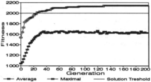
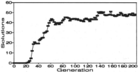
The performance of the algorithm was measured by repeating the experiment ten times. We measured the average and maximal values in the population and the number of solutions present in the population. The results are summarized in Figures 3 and 4.
7 Other Experiments
Although we have not yet attempted to learn models from real world data, QME has been tested on some other small domains. Results for Simple-Spring, Resistor-and-Capacitor-Circuit and P-Controller experiments are presented in Table 1 together with the U-Tube results.
The number of possible finite states and the number of legal states reflect the complexity of a domain. Table 1 also shows the number of positive and negative training examples used in experiments together with the sizes of target models (which were used to generate training examples) and those of induced solutions. In addition, the number of candidate solutions generated during the search, and the fraction of finite states incorrectly classified by the solution are presented.
| Spring | U-Tube | RC-Circuit | P-Control | |
|---|---|---|---|---|
| FiniteStates | 1728 | 20736 | 12192768 | 34666128 |
| LegalStates | 43 | 122 | 48 | 1407 |
| PosExamples | 9 | 17 | 20 | 150 |
| NegExamples | 40 | 78 | 3000 | 3000 |
| Target Size | 3 | 6 | 11 | 12 |
| SolutionSize | 3 | 6 | 12 | 9 |
| CreatedCand | 3400 | 5800 | 7740 | 8940 |
| Error Rate | 0 | 0 | 0.04%o | 0.12%o |
QME was always able to find a model that covers all training examples. During the search only a moderate number of candidates was generated. For the Simple-Spring model a solution identical to the original model was discovered. On the other hand, solutions to the two larger problems were too general and incorrectly recognized a small fraction of illegal finite states as legal ones. The main difficulty is that the large majority of states in these domains is illegal and must be eliminated, while still leaving the sparsely spread legal states.
8 Discussion
A genetic algorithm for learning qualitative models based on the QSIM formalism has been presented. The learning task was considered to be a combinatorial optimization problem based on the maximization of the number of examples covered by a candidate solution and on the minimization of the size of the candidate solution.
We tested our approach on the induction of a model of the U-TUBE system. Learning resulted in a set of models of different specificity and size that explain all given examples. Several solutions equivalent to the original model were discovered as well as more general models and more specific ones.
Coiera [1989] reported that GENMODEL found an overconstrained model of the behavior of the BATHTUB system (similar to the U-TUBE system). However, a model equivalent to the original was not discovered. When applied to the U-TUBE domain GENMODEL, given only six positive examples, produced a model consisting of 14 constraints. On the other hand, in the experiments performed by Bratko et a/. [1991], GOLEM induced a U-TUBE model that is equivalent to the original only in the dynamic sense. Given a legal initial state, this model produces exactly the same behavior as does the original model. However, its decision about legality of several states is inconsistent with the decision of the original model.
Background knowledge can be easily incorporated by introducing suitable "building blocks" into the initial population. We plan to extend our method with the ability of considering corresponding values and introducing new function symbols into the induced models. We also intend to use a meta genetic search t~ tune relevant numerical parameters.
@inproceedings{ijcai1991p193,
  title     = {Qualitative Model Evolution},
  author    = {Varsek, Alen},
  booktitle = {Proceedings of the Twelfth International Joint Conference on
               Artificial Intelligence, {IJCAI-91}},
  publisher = {International Joint Conferences on Artificial Intelligence},
  editor    = {John Mylopoulos and Ray Reiter},
  pages     = {1311--1315},
  year      = {1991},
  month     = {8},
  note      = {Vision},
  url       = {https://ijcai.org/proceedings/1991/193},
}
TY - CPAPER TI - Qualitative Model Evolution AU - Varsek, Alen T2 - Proceedings of the Twelfth International Joint Conference on Artificial Intelligence, IJCAI-91 PB - International Joint Conferences on Artificial Intelligence PY - 1991 SP - 1311 EP - 1315 UR - https://ijcai.org/proceedings/1991/193 ER -Copied
Machine-readable versions of this paper, for tools and AI agents:





