
Hierarchical Genetic Algorithms Operating on Populations of Computer Programs
Proceedings of the Eleventh International Joint Conference on Artificial Intelligence. Machine Learning. Pages 768-773.
© 1989 International Joint Conferences on Artificial Intelligence
Abstract
Existing approaches to artificial intelligence problems such as sequence induction, automatic programming, machine learning, planning, and pattern recognition typically require specification in advance of the size and shape of the solution to the problem (often in a unnatural and difficult way). This paper reports on a new approach in which the size and shape of the solution to such problems is dynamically created using Darwinian principles of reproduction and survival of the fittest. Moreover, the resulting solution is inherently hierarchical. The paper describes computer experiments, using the author's 4341 line LISP program, in five areas of artifical intelligence, namely (1) sequence induction, (2) automatic programming, (3) machine learning of functions, (4) planning, and (5) pattern recognition.
- [Barto et al.,1985] Barto A. G., Anandan, P., and Anderson, C.W. Cooperativity in networks of pattenr recognizing stochastic learning automata. In Narendra, K.S. Adaptive and Learning Systems. New York: Plenum 1985.
- Cramer, Nichael Lynn. A representation for adaptive generation of simple sequential programs. Pro- ceedings of an International Conference on Genetic Algo- rithms and Their Applications. Hillsdale, NJ: Lawrence Erlbaum Associates 1985.
- Davis and Steenstrup 1987]
- Davis, Lawrence and Steenstrup, M. Genetic algorithms and simulated annealing: An over- view. In Davis, Lawrence (editor) Genetic Algorithms and Simulated Annealing London: Pittman 1987.
- DeJong 1987]
- DeJong, Kenneth A. On using genetic algo- rithms to search program spaces. Genetic Algorithms and Their Applications: Proceedings of the Second Interna- tional Conference on Genetic Algorithms. Hillsdale, NJ: Lawrence Erlbaum Associates 1987.
- Fogel et. al. 1966]
- Fogel, L. J., Owens, A. J. and Walsh, M. J. Artificial Intelligence through Simulated Evolution. New York: John Wiley 1966.
- Fujuki 1986]
- Fujuki, Cory. An Evaluation of Holland' s Genetic Algorithm Applied to a Program Generator. Mas- ter of Science Thesis, Department of Computer Science, Moscow, ID: University of Idaho,l986.
- Hicklin, Joseph F., Application of the Genetic Algorithm to Automatic Program Generation. Master of Science Thesis, Department of Computer Science. Moscow, ID: University of Idaho 1986.
- Hinton 1988]
- Hinton, Geoffrey, Neural Networks for Artifi- cial Intelligence. Santa Monica, CA: Technology Transfer Institute. Documentation dated December 12, 1988.
- Holland, John H. Adaptation in Natural and Artificial Systems, Ann Arbor, MI: University of Michigan Press 1975.
- Holland, John H. Escaping brittleness: The possibilities of general-purpose learning algorithms ap- plied to parallel rule-based systems. In Michalski, Ryszard S., Carbonell, Jaime G. and Mitchell, Tom M. Machine Learning: An Artificial Intelligence Approach, Volume II. P. 594-623, Los Altos, CA: Morgan Kaufman 1986.
- Lenat, Douglas B. The role of heuristics in learning by discovery: Three case studies. In Michalski , Ryszard S., Carbonell, J. G. and Mitchell, T. M. Machine Learning: An Artificial Intelligence Approach, Volume I. P. 243-306. Los Altos, CA: Morgan Kaufman 1983.
- Minsky and Papert 1969]
- Minsky, Marvin L. and Papert, Seymour A. Perceptrons. Cambridge: MIT Press. 1969.
- 1988a] Nilsson, Nils J. Action networks. Draft Stan- ford Computer Science Department Working Paper, Octo- ber 24, 1988. Stanford, CA: Stanford University. 1988.
- 1988b] Nilsson, Nils J. Private Communication.
- Schaffer 1987]
- Schaffer, J.D. Some effects of selection pro- cedures on hyperplane sampling by genetic algorithms. In Davis, L. (editor) Genetic Algorithms and Simulated An- nealing London: Pittman 1987.
- Smith, Steven F. A Learning System Based on Genetic Adaptive Algorithms. PhD dissertation. University of Pittsburgh 1980.
- Wilson 1987
- Wilson, S. W. Classifier Systems and the animat problem. Machine Learning, 3(2), 199-228, 1987.
References were extracted automatically from the PDF and may contain errors.
Full text extracted automatically from the PDF; figures, tables and equations may differ. The PDF is the version of record.
1 Introduction
Sequence induction requires developing a computational pro cedure that can generate any arbitrary element in a sequence S = S 0 ,S 1 , ··· ,S., ... given a finite number of specific examples of the values of the sequence. Examples are finding a correct recursive computational procedure for the Fibonacci sequence or finding a polynomial sequence expression of the appropriate order given a finite sampling of the initial values of the sequence. Although induction problems admittedly do not have closed mathematical solutions, the ability to correctly perform induction is widely accepted as a componentofhuman intelligence.
Automatic programming requires developing a computer program that can produce a desired output for a given set of inputs. Examples include finding a computational procedure for solving a given pair oflinear equations a 11 x 1 + a 12 x 2 = b 1 and ~1x1 + a 22 x 2 = b 2 for the real n~mbers ~1 and x 2 , fin~ing a c~m putational procedure for solvmg a gtven quadratic equation ax 2 + bx + c = 0 for complex-valued roots x 1 andx 2 ,and solving trigonometric identities.
Machine learning of a function requires developing a com putational procedure that can rerum the correct functional value for any combination of arguments given a finite number of specific examples of particular combinations of arguments and the associated functional value. An example is the problem of learning the Boolean multiplexer function.
Planning in artificial intelligence and robotics requires find ing a plan that receives information from sensors about the state of various objects in the robotic environment and uses that information to select a sequence of functions to execute in order to change the state of the objects in the robotic environ ment. An example of a planning problem involves generating a general plan for stacking labeled blocks onto a target tower in a specified desired order.
Pattern recognition requires finding a computational proce dure that processes a digitized input image to determine whether a particular pattern is present in the input image.
All of these problems, and many similar problems in artifi cal intelligence and symbolic processing, can be viewed as re quiring the creation of a LISP S-expression (i.e. a computer program, a computational procedure, a robotic plan) com prised of various functions and various atoms appropriate to the given problem domain that returns the desired values (and performs the desired side effects) when presented with a particular combination of input values.
In each case, it would be difficult and unnatural to try to specify the size and shape of the eventual solution in advance. Moreover, attempting such specification in advance narrows the window by which the system views the world and may well preclude finding the solution.
The fitness of any LISP S-expression in a problem environment can be naturally measured by the sum of the dis tances (taken for all the cases in the test suite) between the point in the solution space (whether Boolean-valued, integer-val ued, real-valued, vector-valued, or complex-valued) created by the S-expression for a given set of arguments and the correct point in the solution space. The closer this sum is to zero, the better the S-expression.
As will be Seen, the LISPS-expression required to solve the problem will, in each case, emerge from a simulated evolution ary process which starts with an initial population of randomly generated LISPS-expressions containing functions and atoms appropriate to the problem domain. Predictably, these initial random individual S-expressions will have exceedingly low fitness (when measured by the previously mentioned objective function). Nonetheless, some individuals in the population will be somewhat more fit in the environment than others. Then, a process of sexual reproduction among two parental S-expression selected in proportion to fitness creates offspring S-expressions comprised of sub-expressions ("building blocks") from their parents. The offspring then replace their parents. At each stage, the only input is the fitness of the individuals in the current population. This process tends to produce populations which, over a period of generations, exhibit increasing average fitness in dealing with their environment and which also can robustly adapt to changes in their environment
2 Background
Observing that sexual reproduction in conjunction with Dar winian natural selection based on reproduction and survival of the fittest enables biological species to robustly adapt to their environment, Professor John Holland of the University of Michigan presented the pioneering mathematical formulation of simulated evolution (genetic algorithms) for fixed-length character strings in Adaptation in Natural and Artificial Sys tems (Holland 1975).
Although genetic algorithms superficially seem to only process the particular individual binary strings present in the current population, Holland's 1975 work focused attention on the fact that they actually also automatically process large amounts of useful information in parallel concerning unseen Boolean hyperplanes (called similarity templates or schemata) representing numerous similar individuals not actually present in the current population. Genetic algorithms have a property of"intrinsic parallelism" which enable them to create individ ual strings for the new population in such a way that all the hyperplanes representing similar other individuals are all auto matically expected to be represented (without any explicit computation or memory beyond the population itself) in pro portion to the fitness of the hyperplane relative to the average population fitness. As Schaffer ( 1987) points out, "Since there are very many more than N hyperplanes represented in a population of N strings, this constitutes the only known ex ample of the combinatorial explosion working to advantage instead of disadvantage."
In addition, Holland established that the seemingly unpre possessing genetic operation of crossover in conjunction with the straight-forward operation of fitness proportionate repro duction causes the unseen hyperplanes (schemata) to grow (and decay) from generation to generation at rates that are mathematically near optimal when the process is viewed as a set of multi-armed slot machine problems requiring an optimal allocation of trials so as to minimize losses.
Holland's 1975 work also highlighted the relative unimpor tance of mutation in the evolutionary process and contrasts sharply in this regard with numerous other efforts based on the approach of merely saving the best from among asexual random mutants, such as the 1966Artificiallntelligence through Simulated Evolution (Fogel et. al. 1966) and other work (Lenat 1983, Hicklin 1986).
Representation is a key issue in genetic algorithm work because the representation scheme can severely limit the window by which the system observes its world. However, as Davis and Steenstrup (1987) point out, "In all of Holland's work, and in the work of many of his students, chromosomes are bit strings." String-based representation schemes are diffi cult and unnatural for many problems (DeJong 1987, Smith 1980, Fujuki 1986, Hicklin 1986, Cramer 1985). String-based representation schemes do not provide the hierarchical struc ture central to the organization of computer programs (into programs and subroutines) and the organization of behavior (into tasks and subtasks). String-based representation schemes do not provide any convenient way of representing arbitrary computational procedures or incorporating iteration or recur sion when these capabilities are inherently necessary to solve the problem (e.g. the Fibonacci sequence). Moreover, string based representation schemes do not facilitate computer pro grams modifying themselves and then executing themselves. Moreover, without dynamic variability, the initial selection of string length limits in advance the number of internal states of the system and the computational complexity of what the system can learn.
3 Hierarchical Genetic Algorithms
The LISP programming language is especially well-suited for handling hierarchies, recursions, logical functions, composi tions of functions, self-modifying computer programs, self executing computer programs, iterations, late typing of vari ables and expressions, and complex structures whose size and shape is dynamically determined (rather than predetermined in advance). Because of these features, the LISP programming language allows the creation of "hierarchical" genetic algo rithms for simulated evolution in which the population consists of individual hierarchical LISP $-expressions, rather than strings of characters or other objects (whether of fixed or variable length).
In hierarchical genetic algorithms, the set of possible $ expressions for a particular domain of interest depends on the functions and atoms that are available in the domain. The possibleS-expressions are those that can be composed recur sively from a set of n functions F = ( f 1 , f 2 , ·· · , fn} and a set of m atoms A = ( a 1 , a 2 , ··· , am}. Each particular function fin F takes a specified number z(f) of arguments bl' b 2 , ··· , b~ 0 · For example, the LISP $-expression(+ (cr (- J 1) 1) (cr (- J t+ 1 1) 0))) is an S-expression for the Fibonacci sequence. In this rep resentation, J is the index for the current sequence element and ( crx y) is the sequence referencing function returning the value of the sequence at position x (provided x is between 0 and J -1) or the default value y (if cr is being asked to provide a position of the sequence that is not yet defined).
The operation of fitness proportionate reproduction for hi erarchical genetic algorithms is the basic engine of Darwinian reproduction and survival of the fittest. It is an asexual opera tion in that it operates on only one parental $-expression. The result of this operation is one offspring S-expression. In this operation, if s;(t) is an individual in the population at generation t with fitness value f(s;(t) ), it will be copied into the mating pool for the next generation with probability f(s;{t))/L f(s;(t)).
The crossover operation is a sexual operation that starts with two parental $-expressions. Its result is, for convenience, two offspring $-expressions. Every LISP S-expression can be depicted graphically as a rooted point-labeled tree in a plane whose internal points are labeled with functions, whose exter nal points (leaves) are labeled with atoms, and whose root is labeled with the function (or atom) appearing just inside the outermost left parenthesis. The crosso\!er operation begins by randomly and independently selecting one point in each parent using a uniform distribution. This crossover operation is well defined for any two $-expressions and any two crossover points and the resulting offspring are always valid LISP $ expressions. Offspring contain some traits from each parent.
The "crossover fragment" for a particular parent is the rooted sub-tree whose root is the crossover point for that parent and where the sub-tree consists of the entire sub-tree lying below the crossover point (i.e. more distant from the root of this parent). Viewed in terms of lists in LISP, the crossover frag ment is the sub-list starting at the crossover point.
The first offspring is produced by deleting the crossover fragment of the first parent from the first parent and then impregnating the crossover fragment of the second parent at the crossover point of the first parent. In producing this first offspring the frrst parent acts as the base parent (the female parent) and the second parent acts as the impregnating parent (the male parent). The second offspring is produced in a symmetric manner.
For example, consider the two parental LISP $-expressions below.
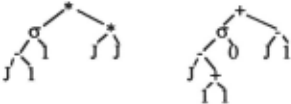
Assume that the points of trees are numbered in a depth-frrst way starting at the left. S oppose that point 2 (out of the 9 points of the frrst parent) was selected as the crossover point for the frrst parent (i.e. the a) and that point 9 (out of the 11 points of the second parent) was selected as the crossover point of the second parent (i.e. the subtraction function- at the right). The two crossover fragments are below.
,,
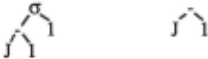
In terms of LISP $-expressions, the two parents are(* ( !l1:. l..1l.Il (* J J))) and(+ (a(- J (+ 1 1)) 0) !.:..1..D.) and the two crossover fragments are the underlined sublists.
The two offspring resulting from crossover are shown below.
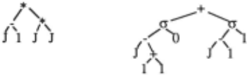
Note that the second offspring above is a perfect solution for the Fibonacci sequence, namely(+ (a(- J (+ 1 1) 0)) (a( J 1) 1) ).
Crossover can be efficiently implemented in LISP using the RPLACA function in LISP (in conjunction with the COPY TREE function) so as to destructively change the pointer ofthe CONS cell at the crossover point of one parent so that it points to the crossover fragment (sublist) of the other parent.
In each of the runs reported herein, between 75% and 80% of the crossover points are restricted to function (internal) points of the tree in order to promote the recombining of larger structures than is the case with an unrestricted selection (which may do an inordinate amount of mere swapping of atoms in a manner more akin to point mutation rather than true cross over).
4 Experimental Results
This section describes some experiments using hierarchical genetic algorithms. The author's computer program, consist ing of 4341 lines of Common Lisp code, was run on a Texas Instruments Explorer II computer with a 25 megaHertz LISP microprocessor chip with 32 megabytes of internal memory. For each experiment reported below, the author believes that sufficient information is provided to allow the experimenllo be independently replicated to produce substantially similar re sults (within the limits inherent in any process involving ran domized selections). Substantially similar results were ob tained on several occasions for each experiment.
4.1.1 Sequence Induction - Fibonacci Sequence
For this experiment, the problem is to induce the computa tional procedure (i.e. LISP S-expression) for the Fibonacci sequence. The environment in which adaptation is to take place consists of the frrst 20 elements of the actual Fibonacci se quence S = 1, 1, 2, 3, 5, 8, 13, 21, 34, 55, ... , 4181, 6765.
The set of functions available for this problem is F = { +, -, a, *} and the set of atoms available is A= {0, 1, J}. For our purposes here we can view each atom as a function that requires no arguments in order to be evaluated. Thus, the combined set of functions and atoms is c = { +, -, a, *, 0, 1, J} having 2, 2, 2, 2, 0, 0, and 0 arguments, respectively. In order to make the experiment more realistic, extraneous func tions or atoms are included in all the experiments reported herein. The multiplication function here is extraneous to a parsimonious solution of this problem. A population of300 in dividuals is used in all examples herein unless otherwise stated. The algorithm begins by randomly generating 300 LISP S-expressions recursively using the items from set C. Ex amples of such random S-expressions included(+ J J), (* 0 ( J 1)), and(*(-(+ J 1) 0) (a J J)).
The raw fitness of an individual LISP S-expression in the population at any generational time step tis I: I P/t)- S.l where S. is the actual Fibonacci sequence element and Ph.(t) is the vhlue returned by $-expression h for sequence positioh j. In this case, the smaller the raw fitness, the closer the match between the performance of the LISP $-expression involved and the actual Fibonacci sequence.
The best $-expression for generation 0 (the initial random population) was(a(-J (a(-J J)O))O) with a raw fitnessof6765. The worst individual had a raw fitness of 28979. The average value of raw fitness was 17621. An adjusted fitness value ~ = 1/(1 +r) is then computed from the raw fitness r for each individual h. A normalized fitness value ~ = aJL ~(ranging between 0 and 1 for each individual) is then computed for each individual. The average value of adjusted fitness for generation 0 was .0001 and the average normalized fitness was .0086. The number of exact matches for the best individual was 1 (out of 20). These predictably poor values for generation 0 serve as a useful baseline for the entire process.
A new population is then created from the current popula tion. This process begins with the selection of a mating pool equal in size to the entire population using fitness proportion ate reproduction (with replacement). In this run and each of the runs reported herein, the number of individuals involved with crossover equals 100% of the population for each generation. When these operations are completed, the new population re places the old population.
The value of average fitness improved (i.e. dropped) from 17621 for generation 0 to 16969 and 15515 for generations 1 and 2, respectively. It then continued to improve monotoni cally to 5928 for generation 10. Between generations 11 and 24, the average fitness oscillated in the general neighborhood of 6000. Then, for generation 25, the value of average fitness improved to 5390. In addition, there was a monotonically improving trend for the fitness of the best individual in the population from generation to generation. The worst individ ual in the population exhibited considerable variability (as is typical) but did improve overall. The average normalized fitness for each generation was very small until generation 16 (when an a very good individual appeared) and thereafter showed a substantial upwards movement.
The number of exact matches for the best individual of each generation started at 1 for generation 0, remained at 1 between generations 1 and 6, dropped to 0 at generation 7, rose to 2 bet ween generations 8 and 13, rose to 18 for generations 14 and 15, rose to 19 for generations 16 through 21. Starting at generation 22, the best individual had a perfect score of 20 matches, namely
(- (+ (cr (+ (- 0 1) J) 1) (cr (+ (- (- 0 1) 1) J) 0)) 0). This S expression equals(+ (cr (- J 1) 1) (cr (- J 2) 0))).
The computer program takes approximately 150 seconds for 300 individuals for 26 generations. The process includes extensive interactive output consisting of two full-color graphs (with mouse-sensitive graph points) and five other windows for monitoring the process.
The number of possible trees increases rapidly with the number of points. This number is dramatically increased by labeling the points of the tree with functions or atoms and is further increased by designating the root. The best S-expres sion in 3,000,000 random initial $-expressions had only 3 matches out of 20. Even if only trees with 13 points are considered, the search space is very large in relation to the 6600 individual LISP $-expressions processed in the 22 generations involved above.
An asexual point mutation operator and an asexual muta tion operator which inserts a randomly generated sub-tree at a randomly selected point were also tested in several runs. No run using either mutation operator and only fitness proportion ate reproduction produced a solution. Moreover, an examina tion of the hereditary history (i.e. LISP audit trail indicating parents, crossover points, mutation points, etc.) of solutions achieved in various runs using crossover revealed that the solution never came about as a result of mutation operation.
The algorithm seems relatively insensitive to the inclusion of extraneous functions and atoms in the repertoire.
4.1.2 Sequence Induction - Cubic Polynomial Sequence
For this experiment, the problem was to induce the computa tional procedure for cubic polynomials such as 1+2J+J2+P. Note that neither the order of the polynomial required nor the size and shape of the computational procedures needed to solve this (and other problems herein) is provided to the problem solver in advance. The same functions and atoms as the Fibonacci sequence were used. Population size was 500. Starting with generation 5, a computational procedure emerged that returned values that exactly matched the actual cubic polynomial for all sequence positions. Similar results were ob tained for a variety of different polynomials. Interestingly, in one run, the program unexpectedly factored the polynomial into a product of factors (J - rk), where the rk were the roots of the polynomial.
4.2.1 Automatic Programming - Pairs of Linear Equa tions
The problem of automatic programming requires developing a computer program that can produce a desired output for a given set of inputs. For this experiment, the problem is to find the computational procedure for solving a pair of consistent non indeterminate linear equations, namely a 11 x 1 + a 12 x 2 = b 1 and 3z 1 X 1 + a 22 xf = b 2 for two real-valued variables. The environ ment consisted of a suite of 10 pairs of equations (to avoid being misled). Without loss of generality, the coefficients of the equations were prenormalized so the determinant is 1. The set of available functions is F = { +,-,*}and the set of available atoms is A= {All, Al2, A21, A22, B1, B2}. The raw fitness of a particular $-expression is the sum of the Euclidian dis tances between the known solution point in the plane and the point produced by the $-expression for all1 0 pairs of equations in the test suite.
The average raw fitness of the population immediately begins improving from the baseline value for generation 0 of 2622 to 632, 341, 342, 309, etc. In addition, the worst individ ual in the population also begins improving from 119051 for generation 0 to 68129,2094, etc. The best individual from gen eration 0 is ( + (- A12 (* Al2 B2)) (+ (* A12 B 1) B2)) and has a raw fitness value of 125.8. The best individual begins improving and has a value of 106 for generations 1 and 2, 103 for generation 3 through 5, 102 for generations 6 through 16, and 102 for generations 17-20. The computational procedure (+ (- A12 (* Al2 B2)) (* A22B1)) appearing in generations 21 and 22 had a fitness value of 62 and differed from the known correct solution only by one additive term -A12. The best individual for generations 23 through 26 is a similarly closeS expression (+ (- A22(* A12 B2)) (* A22 B 1)) with a raw fitness value of 58. Starting with generation 27, a perfect solution for x 1 emerges, namely (- (* A22 B 1) (* A12 B2)). Between generations 27 and 30, the average normalized fitness rises to .39 (as the perfect solution starts dominating).
4.2.2 Automatic Programming- Quadratic Equations
For this experiment, the problem is to solve the quadratic equation x 2 + bx + c = 0 for a complex-valued root. The available functions were multiplication, subtraction, a square root functionS [which returns a LISP complex number, e.g. (S -4) is #C(O, 2)], and a modified division operation % (which re turns a value of zero for division by zero). The environment consistedofasuiteof10quadraticequations(withsomepurely real roots, some purely imaginary roots, and some complex valued roots). A correct solution to the problem emerged at generation 22, namely, the S-expression (- (S (- (* (% B 2) (% B 2)) C))(% B 2)).
4.2.3 Automatic Programming - Trigonometric Identities
For this group of experiments, the problem was to derive various trigonometric identities. This particular group of ex periments yielded a number of unexpected results. The envi ronment consisted of a Monte Carlo suite of 20 pairs of randomly generated X values between 0 and 2TI radians and the value of cos 2X (which is equivalent to 1- 2 sin 2 X). The available functions were SIN, multiplication, and subtraction (with the addition and cosine function were intentionally deleted from the repertoire of available functions). The correct S-expression (- (- 1 (*SIN X) (SIN X)))(* (SIN X) (SIN X))) was obtained after 13 generations in one run and the somewhat more parsimonious correct S-ex pression (- 1 (* (* (SIN X) (SIN X)) 2)) was obtained after 16 generations. In one run with cos 2X, the S-expression (SIN(-(- 2 (*X 2)) (SIN (SIN (SIN (SIN (SIN (SIN(* (SIN (SIN 1)) (SIN (SIN!))))))))))), where 1 is in radians, was obtained as the best individual. This expres sion approximately equals sin (ll/2 - 2X).
4.3.1 Machine Learning- Boolean Multiplexer Function
For this experiment, the problem is to find the Boolean expres sion which gives the correct Boolean output value for a given Boolean multiplexer function. The input to the Boolean multiplexer function consists of k "address" bits ai and 2k "data" bits di and is a string of length k+2k. The value of the multiplexer function is the value (0 or 1) of the particular data bit that is singled out by the k address bits of the multiplexer. For example, for the 6-multiplexer (where k = 2), if the two address bits a 1 a 0 are 11, then the output is the third data bit~· This function has been studied in connection with neural nets (Barto et. a/. 1985) and classifier systems (Wilson 1987).
The combined set of functions and atoms for this problem is C = {NOT, OR, OR, OR, AND, AND, IF, IF, AO, A1, DO, D1, D2, D3 } with 1,2,3,4,2,3,2,3,0,0,0,0,0, and 0 arguments, respectively. Note that the OR, AND, and IF functions appear with varying number of arguments (e.g. 2, 3, or 4). For example, the IF function with 3 arguments is an if-then-else function. The environment consisted of the 2w (where w = k+2k) possible inputs.
Initial random individuals include contradictions such as (AND AO (NOT AO)), inefficiencies such as (OR D3 D3), irrelevancies such as (IF AO AO (NOT A 1) ), and nonsense such as (IF (IF (IF D2 D2) D2) D2). The best individual from generation 0 was (IF AO D 1 D2) with a raw fitness value of 16 (i.e. 16 mismatches out of a possible 64). This individual uses just one of the address bits (AO) to decide whether the output is data line D1 orD2and can never give an output of DOor D3. Nonetheless, in the valley of the blind, the one-eyed man is king.
The average raw fitness of the population immediately begins improving from the baseline value for generation 0 of 29.05 to26.89,25.74, 23.78,22.09, 21.38, 20.13, 19.91,etc. In generation 9 a best individual arises that has only 12 mis matches, namely (IF (IF AO (OR A1 DO)) D3 (IF AO D1 D2)). Note that (IF AO D1 D2) from generation 0 is now embedded as a sub-expression within this new individual. In generation 11, a new best individual arises that has only 8 mismatches, namely (IF AO D1 (IF A1 D2 DO)). The sub-expression (IF A1 D2 DO) contributes substantially to this improved performance because it perfectly deals with the case when AO is NIL (False) by taking either data line D2 or DO as its output (depending on AI). Note also that(IF AO D1 ... ) is partially correct when AO is T (True). In generations 12, 13, and 14, a new individual arises with only 4 mismatches, namely, (IF (IF (AO (OR A1 DO) D3 (IF AO D1 (IF A1 D2 DO)))).
In generation 15, a perfect solution i.e. an individual with 0 mismatches) emerges, namely, (IF (IF AO A1) D3 (IF AO D1
(IF A1 D2 DO)) as a result of a crossover where the unfit sub expression (IF (AO (OR A1 DO))) is replaced by the more fit sub-expression (IF AO A1).
The interpretation of this solution expression is as follows: The output of the multiplexer is D3 if (IF AO A1) is true (i.e. the two address bits are 11). Note that IF function in LISP (unlike the predicate calculus) is equivalent to the AND function. If that is not true, the output is D 1 if AO is true (because the two address bits are necessarily now 01). Note that setting the output to D 1 if merely AO were true in a vacuum is not a correct solution to the problem. However, after (IF AO Al) has been considered (and found to be false), then (IF AO D 1 ... ) is correct. Finally, (IF A1 D2 DO) now handles the case when address bit AO must necessarily be NIL. In this context, the partially correct sub-expression that was around since generation 0, namely (IF A1 D2 DO), sets the output of the multiplexer to D2 if A1 is T (because the two address bits are 10) and, otherwise, it sets the output to DO (because the two address bits are 00).
Note that a default hierarchy emerged here which incorpo rated partially correct sub-rules into a perfect overall proce dure by dealing with ever more specific cases. Although default hierarchies are considered desirable in classifier sys tems (Holland 1986), none emerged in Wilson's (1987) other wise noteworthy experimentS involving classifier systems and the multiplexer.
The perfect solution above arose after processing 4500 individuals. Note that the hierarchical algorithm does not start with any advance information identifiying inputs versus out puts or any advance information about the size and shape of the ultimate solution.
4.3.2 Machine Learning - The Parity Function
For this experiment, the problem is to find the Boolean expres sion for the Boolean parity function. The k-parity function takes k Boolean arguments and returns T if an odd number of its arguments are T and returns NIL otherwise. The exclusive or function and the k-parity function were not realizable by early simple perceptrons (Minsky and Papert 1969) and are, as a result, commonly used as test functions for multi-layered non-linear neural networks. Moreover, these functions yield uninformative schema (similarity templates) with conven tional linear genetic algorithms using fixed length binary strings so that these functions are not realizable with such linear genetic algorithms.
The combined set of functions and atoms used for the 3parity function was C = {AND, OR, NOT, IF, D2, D1, DO} with 2, 2, 1, 3;0, 0, and 0 arguments, respectively. In generation 5, an individual emerged which was correct in all 8 cases, namely (IF (IF D2 DO (NOT DO)) D1 (NOT Dl)).
4.4 Planning
Nilsson (1988a) has presented a robotic action network that solves a problem described to Nilsson (1988b) by Ginsberg in volving rearranging labeled blocks in various towers from an arbitrary initial arrangement into an arbitrary specified new or der on a single target tower. In the experiment here, the goal is to automatically generate a general plan that solves this prob lem.
Three lists are involved in the problem. GOAL-LIST is the list specifying the desired final order in which the blocks are to be stacked in the target tower (i.e. "FRUITCAKE" or "UNI VERSAL"). STACK is the list of blocks that are currently in the target tower (where the order is important). TABLE is the list of blocks that are currently not in the target tower. The ini tial configuration consists of certain blocks in the STACK and the remaining blocks on the TABLE. The desired final confi guration consists of all the blocks being in the STACK in the order specified by GOAL-LIST and no blocks being on the TABLE.
The environment consists of the various different initial configurations ofN blocks in the STACK and on the TABLE. The raw fitness of a particular individual plan in the population is the number of initial configurations for which the particular plan produces the desired final configuration after the plan is executed. The computation of fitness can be significantly shortened by consolidating functionally equivalent initial configurations.
In the problem as stated, three sensors dynamically track the environment in the formulation of the problem. TB is a sensor that dynamically specifies the CAR (i.e. first element) of the list which is the longest CDR (i.e. list of remaining elements) of the list STACK that matches a CDR of GOAL-LIST. NN is a sensor that dynamically specifies the next needed block for the STACK (i.e. the immediate predecessor of TB in GOAL LIST). CS dynamically specifies the CAR of the STACK (i.e. the top block). Thus, the set of atoms available for solving the problem here is A= {TB, NN, CS}. Each of these atoms may assume the value of one of the block labels or the value NIL.
The set of functions available for solving the problem here contains6functionsF= {MS,MT, DU, QUOTE,NOT,EQ}. The function MS has one argument and moves block X to the top of the STACK if X is on the table. The function MT has one argument and moves the top item to the TABLE if the STACK contains X anywhere in the STACK. The iterative function DU ("do until") has two arguments, namely a predicate PRED and some WORK. Both the MS and MT functions have return values, although their true functionality consists of their side effects on STACK and TABLE. The function DU tests the predicate PRED and does the WORK (via the LISP evaluation function EV AL) repeatedly until the predicatePRED becomes T (True). Note that the fact that each function returns some value (in addition to whatever side effects it has on the STACK and TABLE) and the flexibility of the LISP language guaran tees that the DU function can be executed and evaluated for any combination of functions and arguments (however unusual, pointless, or counter-productive). Since individuals in the population will often contain complicated nestings of DU functions and unsatisfiable termination predicates, limits are placed on both the number of iterations allowed (without pre venting any plan from being executed and evaluated).
After about 5 generations, we typically see the emergence of perhaps one plan in the population that correctly deals with the simplest group of cases in the environment (i.e. the cases in which the blocks, if any, in the initial STACK are already all in the correct order and in which there are no out-of-order blocks on top of those blocks). In several runs, the rather parsimonious (DU (QUOTE (MS NN)) (NOT NN)) emerged as a partially correct plan. This plan works by improving a partially correct initial STACK by moving needed blocks (NN) in the correct sequence from the TABLE onto the STACK until there are no more blocks needed to finish the STACK (i.e. the sensor NN is no longer a block).
After about 10 generations, the best single individual in the population is typically a plan that achieves a perfect score. One such plan is (NOT (EQ (DU (QUOTE (MT CS)) (NOT NN)) (EQ (MS (DU (QUOTE (MS NN)) (NOT NN))) (DUNN (QUOTE TB))))). Note that this plan contains a default hierar chy. In particular, the sub-plan (DU (QUOTE (MS NN)) (NOT NN)) comes from an earlier generation (which performed cor rectly for a simple set of cases of initial configurations). This sub-plan is now incorporated as a sub-plan (i.e. a small "build ing block"). Note also that another sub-plan (DU (QUOTE (MT CS)) (NOT NN)) from another individual from an earlier generation correctly deals with the remaining cases by first moving out-of-order blocks from the STACK to the TABLE until the STACK contains no incorrect blocks.
4.5 Pattern Recognition
Hinton (1988) has discussed the problem of translation-invari ant recognition of a one-dimensional shape in a linear binary retina (with wrap-around) in connection with the claim that connectionist neural networks cannot possibly solve this type of problem. In the simplified experiment here, the retina has 6 pixels (with wrap-around) and the shape consists of three consecutive binary 1 's.
The functions available are a zero-sensing function HO, a one-sensing function Hl, ordinary multiplication, and a dis junctive function U. The atoms available are the integers 0, l, and 2, and a universally quantified atom k.
LISP's comparative tolerance as to typing is well suited to pattern recognition problems where it is desirable to freely combine numerical concepts such as positional location (either absolute or universally quantified) and relative displacement (e.g. the symbol 2 pixels to the right) with various combina tions of Boolean tests. The functions U and* so defmed resolve potential type problems that would otherwise arise when integers identify positions in the retina.
In one particular run, the number of mismatches for the best individual of generation 0 was 48 and rapidly improved to 40 for generations 1 and 3. It then improved to 0 mismatches in generation 3 for the individual(* 1 (* (H1 K 1) (Hl K 0) (H1 K 2)) 1 ). Ignoring the extraneous outermost conjunction of two l's, this individual returns a value of the integer 1 if and only if a binary 1 is found in the retina in positions 0, 1, and 2 (each displaced by the same constant k).
5 Robustness
The existence and nurturing of a population of disjunctive al ternative solutions to a problem allows hierarchical genetic algorithms to effectively perform even when the environment changes. To demonstrate this ability, the environment for generations 0 through 9 is the quadratic polynomial x 2 +x +2; however, at generation 10, the environment abruptly changes to the cubic polynomial x 3 + x 2 + 2x + 1; and, at generation 20, it changes again to a new quadratic polynomial x 2 +2x + 1 . A perfect-scoring quadratic polynomial for the first environment was created by generation 3. Normalized average population fitness stabilized in the neighborhood 0.5 for generations 3 through 9 (with genetic diversity maintained). Predictably, the fitness level abruptly dropped to virtually 0 for generation 10 and 11 when the environment changed. Nonetheless, fitness increased for generation 12 and stabilized in the neighborhood of 0.7 for generations 13 to 19 (after creation of a perfect scoring cubic polynomial). The fitness level again abruptly dropped to virtually 0 for generation 20 when the environment again changed. However, by generation 22, a fitness level again stabilized in the neighborhood of 0.7 after creation of a new perfect-scoring quadratic polynomial.
6 Theoretical Discussion
Hierarchical genetic algorithms employ the same automatic allocation of credit inherent in the basic string-based genetic algorithm described by Holland (1975) and inherent in Dar winian reproduction and survival of the fittest amongst bio logical populations in nature. In hierarchical genetic algo rithms, the individuals in the population are LISP $-expres sions (i.e.rooted point-labeled trees in a plane) instead oflinear character strings. The set of similar individuals sharing com mon features (i.e. the schemata) is the hyperspace of LISP$ expressions sharing common features. This infinite set can be partitioned into finite subsets by using the number of points as the partitioning parameter. If the subset sharing common features with a specified value of this parameter is considered, fitness proportionate reproduction causes growth or decay in the size of that subset in the new population in accordance with the relative fitness of the subset to the average population fitness in the same way as it does for string-based linear genetic algorithms (with the associated approximately near optimal allocation of trials). The deviation from this approximately near optimal rate of growth or decay is relatively small if the number of points defining the common feature is relatively small and to the extent that the points defining the common feature are coextensive with one subtree. Thus, the overall effect of fitness proportionate reproduction and crossover is that subprograms (i.e. sub-trees, sub-lists) from relatively high fitness individuals are used as "building blocks" for construct ing new individuals and the search is concentrated for succes sive populations into sub-hyperspaces ofS-expressions of ever decreasing dimensionality and ever increasing fitness.
Acknowledgments
Dr. Thomas Westerdale, Dr. Martin A. Keane, and John Perry made valuable comments on drafts of this paper. Eric Mielke of the Texas Instruments Education Center in Austin signifi cantly improved execution time of the author's crossover operation.
@inproceedings{ijcai1989p123,
  title     = {Hierarchical Genetic Algorithms Operating on Populations of Computer Programs},
  author    = {Koza, John R.},
  booktitle = {Proceedings of the Eleventh International Joint Conference on
               Artificial Intelligence, {IJCAI-89}},
  publisher = {International Joint Conferences on Artificial Intelligence},
  editor    = {N. S. Sridharan},
  pages     = {768--773},
  year      = {1989},
  month     = {8},
  note      = {Machine Learning},
  url       = {https://ijcai.org/proceedings/1989/123},
}
TY - CPAPER TI - Hierarchical Genetic Algorithms Operating on Populations of Computer Programs AU - Koza, John R. T2 - Proceedings of the Eleventh International Joint Conference on Artificial Intelligence, IJCAI-89 PB - International Joint Conferences on Artificial Intelligence PY - 1989 SP - 768 EP - 773 UR - https://ijcai.org/proceedings/1989/123 ER -Copied
Machine-readable versions of this paper, for tools and AI agents:





