Line Labeling and Junction Labeling: A Coupled System for Image Interpretation

1 Introduction

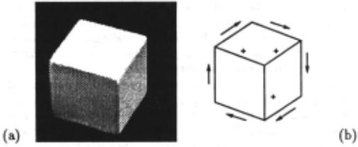
Given a greyscale image of solid, opaque polyhedra with exactly three planes touching at every vertex, we wish to obtain a line labeling for the image. This is illustrated in Figure 1, where (a) is the input image, and (b) is the line labeling produced for that image. The labels used here are based on the well-known work of [Huffman, 1971; Clowes, 1971).

In this task, there are a number of difficulties which are not present in the original formulation of the line labeling problem, or in subsequent work [Waltz, 1975; Malik, 1985). It has generally been assumed that input will be in the form of an idealized line drawing, with each junction correctly pre-classified into one of several types (e.g. T, Y, arrow, etc). The algorithms proposed have been critically dependent on the correctness of this a priori junction classification.

·This work was supported by ONR contract N00014-85K-0692 and ONR grant N00014-89-J-1251 to Donald Glaser of UC Berkeley. The author gratefully acknowledges support from him, and from Jerome Feldman of the International Computer Science Institute in Berkeley. Jitendra Malik of UC Berkeley suggested the application of MRFs to the line labeling problem.

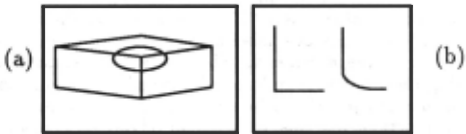
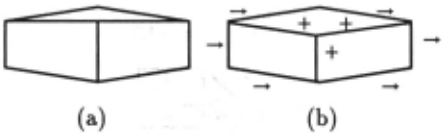
In an actual image of a set of objects, however, junc­ tions of different types may be perceptually quite similar, and thus difficult to classify on the basis of perceptual evidence alone. Figure 2 presents two examples of this. In (a), the circled Y junction is flat enough to be quite similar to a T junction. If the junction were misclassi­ fied this way, the classical line labeling schemes would be worthless. In (b), we see two junction types taken from [Malik, 1985), an extension of early line labeling work to cover the case of piecewise smooth curved objects. The two junction types are perceptually very similar, but place different constraints on the labels of the in­ coming edges. As Malik points out, it is probably asking too much of a separate front-end process to be able to consistently distinguish these.

Thus, quite apart from issues of edge detection and junction detection, this problem of the perceptual similarity of junction types must be addressed by any work which seeks to provide an account of line labeling from images.

2 A Coupled System

The approach taken by this work is to reformulate the line labeling problem in terms of a coupled probabilistic system. Under this scheme, we do not assume correctly pre-classified junctions, as earlier work has. Instead, the issue of perceptual similarity of junction types is ad­ dressed by labeling both lines and junctions. Once lines and junctions are detected, external evidence for partic­ ular junction and line labels is extracted from the image, and this, together with prior probabilities for given con­ figurations of junction and line labels, gives us a poste­ rior distribution over all possible labelings. The idea is to have the system arrive at the labeling with the maxi­ mum a posteriori probability.

This provides a solution to the problem of perceptual similarity of junction types, since any junction in the image which is not clearly of a single junction type will provide weak evidence for all possible labels. For ex­ ample, in Figure 2(a), the circled junction will provide weak evidence for both the "T" label and the "Y" label. The "Y" label will eventually be chosen since it is more consistent with the rest of the image, i.e. because there exists a resulting overall labeling with higher a posteri­ ori probability than any overall labeling in which that junction is labeled as a "T". Note that since the a poste­ riori distribution over labelings is derived through Bayes' rule from the a priori distribution, we are actually let­ ting the prior probabilities of particular configurations of line and junction labels help us determine the label for junctions like this, rather than relying on perceptual evidence alone.

Line labels are determined in the same fashion.

3 Markov Random Fields

Markov random fields (MRFs) are used to implement the above ideas. This formalism has found several uses in machine vision recently (Cross and Jain, 1983; Geman and Geman, 1984; Chou and Raman, 1987; Cooper, 1989]. Before proceeding to outline the details of the system, we present a brief introduction to MRFs, as used here.

Let S be a set of sites connected through an undi­ rected graph, called the neighborhood graph, and let X = {X,, s E S} be a set of random variables indexed by S. Adjacent vertices in the graph correspond to neigh­ boring MRF elements. We assume, without loss of gen­ erality, that there exists a state space (or label space) L common to all the variables, such that the value w, of X, is in L. The term w denotes an assignment of some value from L to each element of X, and is referred to as a configuration.

X is a Markov random field if and only if the proba­ bility distribution P(X = w) is a Gibbs distribution

L---- __ .J

Figure 3: System Architecture

where T is the temperature, U is an energy . term, and Z is a normalizing constant. U is obtained by summing over applicable clique potentials; it is through assigning potentials to cliques 1 in the neighborhood graph of the MRF that one specifies constraints governing local label configurations. Each time a clique matches a subgraph of the neighborhood graph, its clique potential is added to the sum U.

In the work presented here, we wish to take into ac­ count not only the prior probabilities of particular con­ figurations, but also external evidence. The external ev­ idence for a particular label w, at a sites after an obser­ vation 0, is given by the likelihood P(O,Iw,). We make the assumption that these likelihoods are conditionally independent. This allows us to derive the following for­ mula for the posterior Gibbs energy after an observation 0:

where the Vc 's are the clique potentials.

(Chou and Raman, 1987] present a deterministic method, the "Highest Confidence First" (HCF) algo­ rithm, for constructing a configuration with a local min­ imal a posteriori energy measure, giving an estimate to the configuration with maximal a posteriori probability P(wiO). The basic intuition behind the algorithm is that initially, all nodes take the null label, and after that, the first sites to be labeled should be those for which the evi­ dence is most decisive in favor of a particular label. HCF tends to provide fast convergence, requiring an average of around one update per node. This is the algorithm used in the work presented here.

4 Architecture

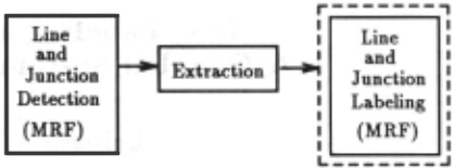
The architecture of the line and junction labeling system is presented in Figure 3. It consists of three stages: line and junction detection, extraction of lines and junctions from the image, and line and junction labeling. The final stage, highlighted with a dotted outline in the figure, is the coupled system that this paper focuses on.

4.1 Detection and Extraction of Lines and Junctions

The detection and extraction mechanisms are covered in detail in (Regier, 1990]. Because of considerations of space, only a brief overview of their operation is pre­ sented here.

1 Recall that a clique is a completely connected subgraph.

4.1.1 Detection of Lines and Junctions

The line and junction detection mechanism accepts a greyscale image of trihedral objects on a dark back­ ground, and produces an array of labels, such that each pixel has been labeled as belonging to either the fore­ ground, the. background, a line of one of 12 orientations, or a junction. This stage is implemented as an MRF.

4.1.2 Extraction of Lines and Junctions

The line and junction extraction mechanism is respon­ sible for translating the output of the first stage into a format suitable for the final one. It accepts as input the pixel-based array of labels computed by the detection mechanism, and produces a neighborhood graph for the line and junction labeling MRF, in which nodes will rep­ resent individual junctions and lines, rather than pixels. It also outputs likelihoods for the various labels of the final MRF. This is done by searching through the pixel­ based output of the first stage, looking for individual junctions and lines. It must then

• Create a junction node for each junction found.
• Create a line node for each line found.
• Set up the neighborhood graph so that each junction node is connected to the line nodes that correspond to lines touching that junction, and so that each line node is connected to the two junction nodes corre­ sponding to the junctions which that line touches.
• Produce likelihoods for the various node and junc­ tion labels in the final MRF.

4.1.3 Line and Junction Roles

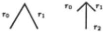
Figure 4 illustrates the roles that lines may play rel­ ative to junctions. There are three possible roles, r0 , r1, and r2, which are assigned as shown in the figure. This assignment is easily done by measuring the angles between adjacent lines at a junction, as follows:

ro is that line for which the clockwise arc dis­ tance to the next line is greatest, r 1 is that next line, and r2 is the next line after that. If there are only two lines meeting at the junction, r2 is null.

These roles serve to let us differentiate one line from another at a junction. This will be crucial when design­ ing cliques for the MRF itself. Note that we do not assign junction labels to junctions at this point; that is done by the MRF. The idea behind this is to give us enough in­ formation to solve the labeling problem without rigidly classifying a given junction prematurely.

8-J

.

.

.

.

There are also roles relative to lines. The extraction mechanism assigns a role to each of the two junctions that a given line connects: these are j 0 and j 1 . There is no particular significance to the numbering here; it is important simply to keep the two distinct. This, to­ gether with the other connectivity information described above, is enough to allow us to build the neighborhood graph for the MRF, which will be presented below.

4.1.4 External Evidence

There is one last thing the extraction mechanism must do: determine the evidence for each of the possible junc­ tion and node labels for each node in the MRF being built. The evidence is currently based on relatively ad hoc personal judgments of what would be appropriate likelihoods, given a particular feature of the image. The values given here have consistently yielded good results.

The label set for junctions is

In the determination of likelihoods for these labels, we examine two cases, depending on the number of lines at a given junction:

Two lines: In this case, the junction has to be an "L", so we set P(O,IL) = 0.9, and set P(O,IA) = 0.01, A E {Y, T, Arrow}.

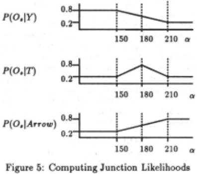
Three lines: In this case, we let a be the largest clockwise arc distance from any of the three lines to the next, and compute the likelihoods for each of the three­ line labels as a function of a, as shown in Figure 5. We also set P(O,IL) = 0.01.

The label set for lines is

i.e. lines can be labeled as either convex, concave, or occluding.

Note: It is important to point out that this line label set is not identical to the original Huffma.n/Clowes for­ mulation. In particular, in the case of occluding edges, the original formulation marked which side of the edge the foreground of the object was on; this label set does not capture that distinction. Thus, we have a collapsed label set, and the solutions found are underspecified in the sense that they do not indicate what is being oc­ cluded by what. The decision was made to use this label set since it simplified the graph structure of the final MRF somewhat. Current work is directed at updating this system so as to capture the missing distinction.

Given this, it is straightforward to compute reason­ able likelihood estimates for the line labels. For a given line, we let {3 be the fraction of the length of the line which borders the background; this is computed during the line-tracing process described above. Then

This reflects the fact that if the edge is either convex or concave, we know it will not border the background, while if it is an occluding edge, it may or may not.

4.2 Line and Junction Labeling

As there are separate label sets for lines and junctions in the line and junction labeling MRF, this is in fact a coupled MRF. We consider first the structure of the neighborhood graph 2 for this MRF, and then the cliques used.

4.2.1 The Neighborhood Graph

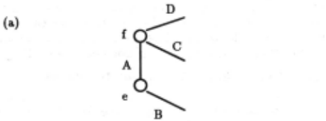
Figure 6 should serve to give a feel for the interplay between junction nodes and line nodes in this coupled system. Figure 6(a) shows a portion of some trihedral object, with two junctions and four edges shown.

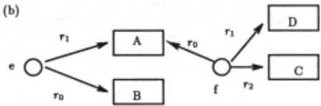
Figure 6(b) indicates which line nodes are neighbors of the two junction nodes, e and f. As described above, the structure of a junction node's neighborhood reflects the structure of the junction in the original image, in that the roles (ro, r1, r 2) are filled appropriately. For example, since the clockwise arc distance from B to A in (a) is greater than that from A to B, junction e's r0 neighbor is B.

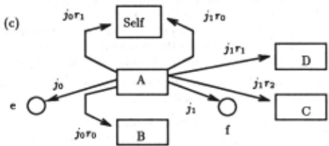
Figure 6(c) indicates which nodes are neighbors ofline node A. Recall that junctions are assigned roles relative to lines, as well; junction e fills role j 0 relative to line A while junction f fills role i1·

Note that line nodes also have, as immediate neigh­ bors, the neighbors of neighboring junction nodes. Thus, the graph constructed by the extraction process also causes line node A to have, as neighbors, each of the line nodes which play roles relative to A'sjunction neighbors. The neighbor filling the ioro role for A is that line which fills the ro role for A's io neighbor. This is line node B.

Under this scheme, one would expect A's j 0r 1 neighbor to be A itself, since the r 1 neighbor of A's io neighbor (e) is A. Instead, the fact that a particular role of A is filled by A itself is encoded by having the corresponding neighbor of A be a special node permanently labeled "Self". I.e. the "Self' node denotes the fact that a node's neighbor is meant to be the node itself. This is Since each line node has two junction neighbors, and since each of these junction neighbors has the original line node as a neighbor, the "Self' node is pointed to twice by each line node in the system.

2 Recall tha.t this is the gra.ph over which the MRF is de­ fined. "Neighbors" a.re a.dja.cent nodes in this gra.ph.

4.2.2 Cliques Used in Line Labeling

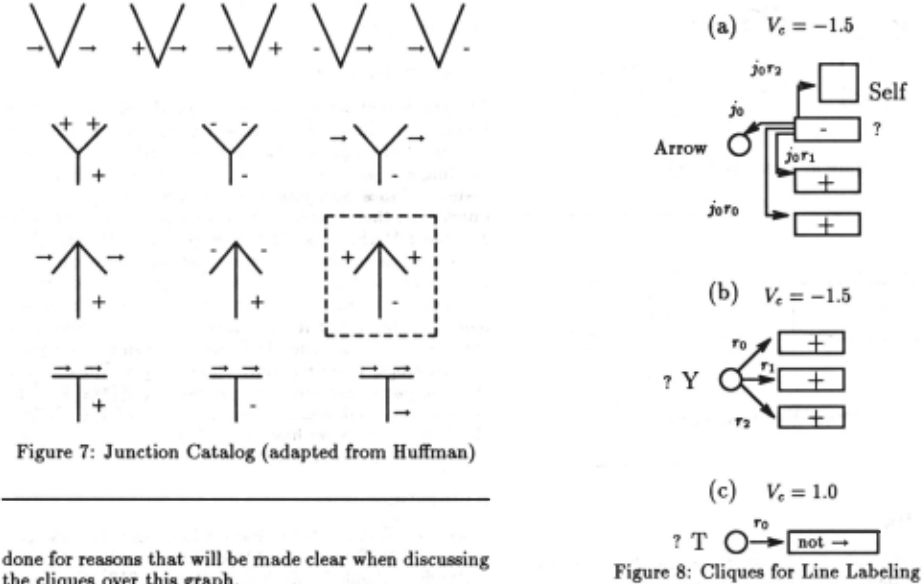
Figure 7 presents the junction catalog which the cliques of this MRF embody. It has been adapted from the original, as we are currently not capturing the direc­ tionality of occluding edges.

Figure 8 presents three sample cliques from the set used here. The node being currently examined is marked by the symbol "?" in each of these. As is usual in the MRF formalism, we try to match each clique against subgraphs of the neighborhood graph.

Figure 8(a) expresses the knowledge that if the current line is in role r2 relative to a junction which has been labeled "Arrow", and if roles r 1 and ro of that junction are lines which have been labeled "+", then it is favored 3 that this line node take on the label "-".

Note how the "Self' node is used. We can check to see if the r2 neighbor of the current node's io neighbor is the current node itself, simply by checking to see if the label on the jor2 neighbor is "Self'. It is crucial to be able to do this, since we need to be sure that the line node we are currently examining is in fact the middle line in an arrow junction. It is, if the io neighbor is labeled "Arrow", and the ior2 neighbor is labeled "Self" .

Referring back to Figure 7, and focusing on the junc­ tion highlighted by a dashed outline, we find that the clique corresponds to the assertion that the middle branch of the arrow should be labeled "-" if the junc­ tion has been labeled as an arrow, and if the other two branches of the junction have been labeled "+". Since this clique covers only junctions which are in relation io to the line in question, we require a similar clique to take care of the corresponding case when the junction fills role JI.

3 Recall equations 1 a.nd 2. In general, a low value for a. clique potential indicates tha.t the corresponding clique is a. relatively acceptable (probable) configuration, while higher values indicate less likely configurations.

While considerations of space preclude the inclusion here of a complete listing of the cliques used by the sys­ tem, most are of the type shown in (a), and encode very specific pieces ·of knowledge from the catalog, regarding what line labels are acceptable in what configurations.

Figure 8(b) encodes the knowledge that if all three lines touching a junction are "+", it is appropriate to favor labeling the junction "Y". Conversely, (c) encodes the knowledge that if the line filling the role ro for some junction is labeled something other than "--+", the junc­ tion should probably not be labeled "T".

It is the inclusion in the system of cliques of this latter sort, governing the appropriateness of particular junc­ tion labels, that makes this work something more than just an MRF implementation of a standard line-labeling algorithm. Through these cliques, the system is able to perform junction labeling which is not just a direct re­ flection of the evidence, so that ambiguous or misleading evidence can be overcome, resulting in a globally consis­ tent solution.

5 Results

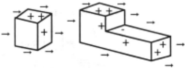
Figure 9 presents correct labelings produced by the system for a pair of trihedral objects. 4

In both cases, the number of node updates required was equal to one per node. Recall that the HCF algo­ rithm first updates those nodes which have strong evi­ dence in favor of a particular label. Thus, "L" junctions and occluding edges tend to be marked first, as there is always strong evidence for each of them. 5 These deci­ sions then influence the other choices, eventually result­ ing in a complete labeling.

More interestingly, Figure 10 presents a situation in which misleading evid~nce (the apparent "T" junction in (a)) is outweighed by constraints placed on the junc­ tion label by the adjacent line labels. Thus, the solu­ tion arrived at in (b) is one in which what looked like a "T" junction has been labeled as a "Y'' junction. 6 This extreme case indicates the system's ability to overcome the problem of perceptual similarity of different junction types, since in this example, a junction which had evi­ dence identical to that for a "T" was labeled as a "Y'' since that was the node label which resulted in an overall labeling with maximum a posteriori probability.

As one might expect, the ''Y'' junction is the last to be labeled, as it is the identity of the three convex lines that touch it that force it to take that label (recall Figure 8(b) and (c)). This is in contrast to the first figure in Figure 9, in which the "Y" had strong evidence, and was labeled relatively early.

4 1nput to the coupled MRF was constructed by hand for the second of the two objects shown, on the basis of what the extraction mechanism would have produced for such an object. ·

sThe presence of only two lines at a junction is strong evidence for an L, and the presence of a stretch of background bordering an edge is strong evidence for an occluding edge (though an occluding edge need not border the background).

6 lnput to the MRF was constructed by hand for this case as well.

6 Conclusions

The problem of perceptual similarity of different junction types, in producing a line labeling from a real image, is addressed through a system which performs both line labeling and junction labeling, in a coupled probabilistic system. Lines and junctions are first detected in the image, and then extracted and used to build a graph for a coupled MRF. This MRF then produces the labeling.

Extensions to this work are currently under consider­ ation. Among the extensions being looked into are (a) marking occluding edges for directionality, ·which will require some minor modifications of the neighborhood graph structure for the MRF, and (b) using other junc­ tion catalogs, covering more than simply trihedral ob­ jects. In particular, the junction catalog of [Malik, 1985] has features that seem to require some of the abilities of this system, as we have seen. This would thus be an appropriate direction for extension.