
Visual Interpretation of Lambertian Surface Deformation
Proceedings of the Twelfth International Joint Conference on Artificial Intelligence. Vision. Pages 1299-1303.
© 1991 International Joint Conferences on Artificial Intelligence
Abstract
This paper considers the interpretation (as a three-dimensional velocity field) of the changing intensity pattern induced by a smoothly deforming Lambertian surface of uniform albedo illuminated by a distant point light source. The requisite "Intensity Rate Constraint" which is derived contains no terms relating to the tangential components of surface velocity, so the determination of the velocity field is ill-posed, exhibiting a form of "Aperture Problem". A stretch-based regulariser is applied to enable estimation of the velocity field and tests with synthetic data show a requirement for high accuracy.
- [Blake et al., 1985] A. Blake, A. Zisserman, and G. Knowles. Surface descriptions from stereo and shading. Image and Vision Computing, 3(4) :183-191 , 1985.
- [Cameron-Jones, 1988] R.M. Cameron-Jones. Visual in- terpretation of cylindrical deformation -a sideways look at contour motion! In Proceedings of the Fourth Alvey Vision Conference, pages 135-140, 1988.
- [Cameron-Jones, 1990] R.M. Cameron-Jones. Visual in- terpretation of lambertian surface deformation. Sub- mitted as Ph.D. thesis, 1990.
- [D'Haeyer, 1986] J. D'Haeyer. Determining motion of image curves from local pattern changes. Computer Vision, Graphics, and Image Processing, 34:166-188, 1986.
- [Horn and Schunck, 1981] B.K.P. Horn and B.G. Schunck. Determining optical flow . Artificial Intelligence, 17:185-203, 1981.
- [Horn, 1986] B.K.P. Horn. Robot Vision. MIT Press, 1986.
- [Jansson and Johansson, 1973] G . Jansson and G. Jo- hansson. Visual perception of bending motion. Per- ception, 2:321-326, 1973.
- [Koenderink and van Doorn, 1986] J .J. Koenderink and A.J. van Doorn. Depth and shape from differential perspective in the presence of bending deformations. J. Opt.Soc.Am.A, 3(2):242-249, 1986.
- [Longuet-Higgins and Prazdny, 1980] H.C. Longuet-Higgins and K. Prazdny. The interpretation of a moving retinal image. Proceedings of the Royal Society of London B, 208:385-397, 1980.
- [Shulman and Aloimonos, 1988] D. Shulman and J . Aloimonos. (non-)rigid motion interpretation: A regularised approach. Proceedings of the Royal Soci- ety of London B, 233:217-234, 1988.
- [Subbarao, 1988] M. Subbarao. Interpretation of Visual Motion: A Computational Study. Pitman, 1988.
- [Weatherburn, 1930] C.E. Weatherburn. Differential Geometry of Three Dimensions, volume 2. Cambridge University Press, 1930.
- [Weatherburn, 1931] C.E. Weatherburn. Differential Geometry of Three Dimensions, volume 1. Cambridge University Press, 1931.
References were extracted automatically from the PDF and may contain errors.
Full text extracted automatically from the PDF; figures, tables and equations may differ. The PDF is the version of record.
1 Introduction
This paper considers a problem in the field of non-rigid motion interpretation. Whereas motion has often been presumed to be merely a cue as to surface structure, as perhaps implied by the phrase "structure from motion", this work takes the stance that in a dynamic world where objects may be in relative, even non-rigid motion, the motion of a world point is i~self of interest. The prob lem addressed here is that of the interpretation (as a three-dimensional velocity field) of the changing inten sity pattern induced by a smoothly deforming Lamber tian surface of uniform albedo illuminated by a distant point light source. Thus, the surface viewed deforming is presumed to accord with the most common assumptions in the field of shape from shading (see e.g. [Horn, 1986]), - the image intensity of a surface point is presumed to vary in a known manner with the angle between the sur face normal and the light source direction. Hence, if the surface deforms such that this angle changes, the in tensity of the (changing) corresponding image point will also change, and the assumption used to derive the "Mo tion Constraint Equation", first proposed in [Horn and Schunck, 1981], and since used to underpin most work in visual motion interpretation, will be broken.
*The author wishes to acknowledge the financial support of the SERC during the early part of this work, the Depart ment for continued use of its resources, the supervision of Drs. R.B.Fisher and J.C.T.Hallam, the comments of L.D.Cai and H.W.Hughes, and the photography of D.Howie.
However, here it is presumed that the instantaneous shape of the deforming surface region may be determined by the application of shape from shading within a bound ing contour, as analysed in [Blake et al., 1985]. Similarly the full three-dimensional velocity is presumed known at identifiable feature points on the bounding contour from combined stereo and motion. This will enable the esti mation of the three-dimensional velocity along the entire bounding contour using a method such as that proposed in [Cameron-Jones, 1990]. Thus, the problem remaining is that of estimating the three-dimensional velocity field over the surface region from the intensity rate, given the velocity on the bounding contour and the static infor mation.
The derived "Intensity Rate Constraint," which re lates the change in intensity at an image point to the mo tion of the surface, contains terms relating to the normal velocity component at the point, but not the tangential components of the velocity. Hence the determination of the three-dimensional velocity field is an ill-posed prob lem, and the application of a regularisation approach using a stretch-based criterion is proposed. The choice of regulariser was motivated by a psychological study of human observation of objects in motion [Jansson and Jo hansson, 1973] which suggested that a distinction should be made between bending and stretching modes of non rigidity, corresponding to deformations in which internal lengths (e.g. those along a surface) are preserved or al tered respectively.
Previous work on continuous non-rigid motion in cludes the extension in [Subbarao, 1988], of the classical rigid motion continuous time optic flow interpretation work of e.g. [Longuet-Higgins and Prazdny, 1980], and [Koenderink and van Doorn, 1986] in which bending mo tion of a surface approximated, with a difference geom etry approach, by hinged planar facets was considered. However, the work most related to that of this paper is [Shulman and Aloimonos, 1988], which proposed a gen eral regularisation framework for the determination of (non-)rigid motion from a changing intensity pattern. The technique proposed here and most previous work may be regarded as special cases of this framework but the approach of this work, which was developed indepen dently, is quite distinct in its use of a coordinate system set in the surface. This enables the form of the con straint relating the image intensity change to the world
where
- I is the image intensity (assuming appropriate sen sor calibration)
velocity to be clarified in a manner which is not possible in the conventional Cartesian coordinate system.
The subsequent sections of this paper will show the derivation of the "Intensity Rate Constraint" and the estimation of the velocity field from synthetic data using the method proposed.
2 The Intensity Rate Constraint
This section shows that for a deforming Lambertian sur face of constant uniform albedo (viewed orthographically and illuminated by an infinitely distant point source), the local image intensity rate is independent of the tan gential components of surface velocity, depending only on the normal component of surface velocity, the in stantaneous shape and the illumination. The derivation of this intuitively obvious, but (as far as the author is aware) hitherto unproved fact is simplified by the use of a coordinate system set in the surface, rather than the Cartesian system customarily employed in the vi sual analysis of motion. This coordinate system is re tained in subsequent sections to emphasise the form of the constraint underlying the interpretation of the in tensity rate, although a transformation into a Cartesian system could be preferable in a practical application.
2.1 Problem Definition
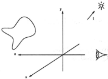
It is desired to derive an expression for the temporal intensity derivative at a point in a changing intensity image, which is the orthographic projection along the z axis of an arbitrarily smoothly deforming smooth surface of constant uniform albedo Lambertian reflectance, illu minated by a point light source at infinity. (See Figure 1).
2.2 Static Image Intensity
For a Lambertian surface, at any instant, the image in tensity corresponding to a point on the surface, will be:
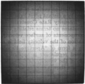
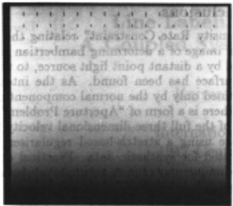
Figure 3: Intensity displayed as a function of lines of curvature parameters
- p is the surface albedo, hereafter absorbed into 1 for convemence
- 1 is the light source vector
- n is the unit normal vector on the surface
2.3 Surface Coordinate System
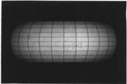
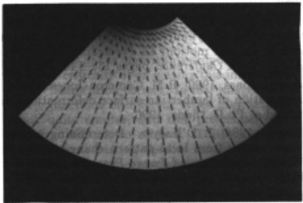
The derivation will presume that the surface has been parameterised (in the form r( ex, /3)) by its lines of cur vature and that all relevant quantities such as image in tensity may be considered as functions of ex and /3, the parameters of the visible point corresponding to the im age point . An example of this is illustrated in Figures 2 and 3, where part of a uniform albedo toroidal sur face (illuminated by a point source behind the viewer) is parameterised by its lines of curvature (as added to the 2:- y plane image) , and the intensity as a function of these parameters illustrated below (with the lines of curvature now forming a rectangular grid).
The choice of parameterisation simplifies the First Fundamental Form (see e.g. [Weatherburn, 1931] for more on differential geometry if required) to:
and the Second Fundamental Form to:
It will also be useful to define the quantity
which represents the surface area per unit area of pa rameter space.
2.4 Derivation
Given the previous expression for the image intensity at a point, knowing that the light source is fixed, and presuming the surface reflectivity to be unchanged in motion, the change in intensity at the changing image point corresponding to a given point on the surface is :
Substituting for the change in the unit normal vector (from e.g. [Weatherburn, 1930]) gives:
where the vector fields v (translational velocity) and n are defined on the surface, and V is defined as:
Considering the full and partial first-order derivatives of image intensity:
Hence
where
- i is the intensity rate at a fixed image point
- Val is the 3-D gradient of the intensity.
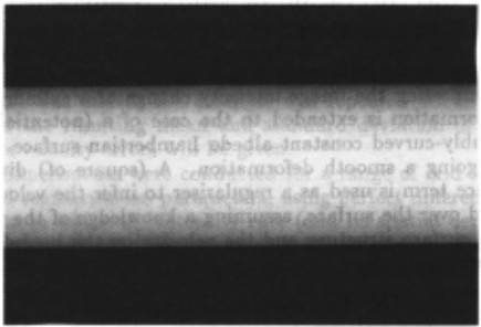
The latter concept may seem rather odd given that the intensity image is two-dimensional! It should be re garded as expressing the projection. In this case, (ortho graphic projection in the z direction) , movement in the z direction will leave the image unaffected as the intensity gradient is zero \n this direction. In the case of per spective projection, contraction towards, or expansion from, the point of projection is special in that a sur face element remains in correspondence with an image plane element. A cross-section of the conceptual three dimensional intensity resulting from the toroidal surface previously illustrated is shown in Figure 4. The terms involving tangential components of velocity in 5 may be eliminated by considering the expansions of the terms, using the basis (ra, rp, n) :
Thus:
by substitution.
Hence
Considering the other term:
Hence
Thus, on collecting the above expressions and can celling the tangential velocity terms, 5 becomes -
The Intensity Rate Constraint :
The intensity rate constraint and the motion con straint equation [Horn and Schunck, 1981], used in the calculation of image flow, are closely related and the for mer exhibits a scaled up form of the "Aperture Problem" associated with the latter, as there are two components of tangential velocity to be indeterminate. Further dis cussion of the new constraint, analytical examples of sur face deformations satisfying it, and a yet more general form may be found in [Cameron-Jones, 1990].
3 Interpretation of Smooth Surface Deformation
In this section the method of [Cameron-Jones, 1988] for interpreting the image intensity change of a cylindrical deformation is extended to the case of a (potentially) doubly-curved constant albedo Lambertian surface un dergoing a smooth deformation. A (square of) diver gence term is used as a regulariser to infer the velocity field over the surface, assuming a knowledge of the ini tial surface structure and the velocity on the bounding contour.
3.1 The Divergence-Based Regulariser
It was shown in the previous section that the intensity rate at a point in an image of a deforming constant albedo Lambertian surface is related to the normal ve locity and its derivatives by the intensity rate constraint 6. It has been proposed in [Cameron-Jones, 1988] that in a special reduced dimensional case of surface motion, equivalent to curve motion in the plane, the velocity field over the surface may be estimated by the application of a stretch-minimising regulariser, as used in [D 'Haeyer, 1986] for determining image curve motion. When con sidering the generalisation of this method to the unre stricted form of smooth surface deformation, the most straightforward approach is to choose a regularisation term which is again a measure of surface stretching, and apply it to the full form of the intensity rate constraint.
The form of this regulariser should be such that it is zero in the case of a pure bending motion and hence the regularisation will yield the correct solution given correct input data representing this significant case. In a pure bending motion the surface dilatation and shear are both zero, hence terms representing either or both seem plau sible candidates. The dilatation (per unit area) is mea sured by the divergence, a differential invariant , which has the prerequisite property of depending upon both tangential and normal velocities and (as will be shown below) is mathematically convenient for considering the limiting case of ideal input data where A may be made very small. Thus the (square of) divergence was used as the regulariser in this work; however, if a similarly appropriate shear-based term were found it might yield correct results in some other interesting cases.
Thus, the velocity field is chosen by minimising (with respect to v) the following integral over the surface, (sub ject to the known von the bounding contour) :
As commented above, this method should yield the correct velocity field in the case of a pure bending mo tion of a surface (which is completely visible and un shadowed), independent of the magnitude of A. A fur ther significant case is that in which the surface is un dergoing a uniform expansion (with everywhere constant divergence) , and A is sufficiently small that the regular isation results in minimising the (square of) divergence term over the surface, subject to the normal velocity found from the intensity rate constraint and the known velocity on the bounding contour. In this case the "di vergence theorem" (page 239 of [Weatherburn, 1931)) may be applied to the known velocities to show that the minimisation is consistent with the correct motion being found.
The divergence theorem states that for a closed curve on a surface (arclength s), letting m be the unit vector tangential to the surface and normal to the curve in the direction out of the enclosed region, the surface integral of the divergence of a vector quantity, such as v is given thus:
Hence the integral of the divergence over the surface may be found from the normal velocity (which is found from the intensity rate constraint) and the known ve locity on the bounding contour, which are constraints upon the minimisation of the integral of the squared di vergence. Consequently the minimisation of the integral of the square of the divergence is done subject to this (implicit) constraint and hence the result of that min imisation will be the correct uniform value of divergence and thus the correct motion field.
The formal minimisation of the regularised problem may be performed by applying the calculus of variations to the integral and the resulting three coupled second order partial differential equations may be solved nu merically over a bounded surface region, given the ve locity on the bounding contour. For further details and more extensive results than will be presented here see [Cameron-Jones, 1990).
3.2 Application Results
The method was tested on data representing two deform ing surfaces: ( 1) a bending circular cylindrical region (as used in [Cameron-Jones, 1988] in which the deformation was restricted to being cylindrical, and hence one di mension of the problem ignored) and (2) an expanding, rotating and translating toroidal region. For simplicity, results are presented for only one deformation of each of these surfaces with only a a few variations of the input.
The first, that of the circular bending motion is illus trated in Figure 5. The surface, as a function of the surface coordinates and time, is given by the expression:
In the example used, the surface region with r = 300, r = 80, 01 and j3 in the range [-240, 240), (both sampled every 30) was viewed from the z direction, at timet = 0. (All dimensions are in pixels. In the case of orthographic projection, this appears a natural unit) . The albedo was 255, and the light source vector at (0.3, 0.3, 0.95).
The second case, that of the toroidal region expansion, rotation (about the z axis) and translation, (viewed from the y direction), is illustrated in Figure 6.
The surface as a function of the surface coordinates ana time is given (at time t = 0) by:
In the example used, the surface region with a = 200, r = 150, e = 0.05, w = 0.07, v., = 10, a in the range [-0.8, 0.8], and /3 in the range [1.2, 2.8] (both sampled every 0.1) was viewed from the y direction, at timet = 0. The albedo was 255 and the light source vector at ( -0.3, 0.9, -0.3).
The two types of motion were both chosen to be cases in which the intensity at the (changing) image point corresponding to a moving point of the viewed surface changes; thus the standard assumption that image flow is equivalent to optic flow does not hold. In the toroidal example, if the rotation is set to zero, the assumption does hold (and the method proposed in this section still works).
The results which will be given are in the form of root mean square ( rms) velocity errors, (calculated over the points at which the velocity is determined). The error at each individual point is the magnitude of the vector which is the difference between the (known) true and estimated three-dimensional velocity. In all cases where noise was added, the example was repeated 100 times and the resulting mean and standard deviation of the rms velocity errors will be given.
Experiments were conducted for a range of grid sizes and regularisation parameters, using perfect differential data in which the intensity rate (and its spatial deriva tives) and velocities are exactly known, using data in which these were found using temporal and spatial finite difference approximations, and experiments in which noise was added. For full details see [Cameron-Jones, 1990].
Results will be given here for the cases of grids of 16 x 16 increments, as depicted in the figures, using a regularisation parameter of 10- 4 , in the noisy finite time increment case. The velocity rms errors should be com pared with:
- The rms true velocities over the cylindrical and toroidal surfaces: 9.87864 and 11.1511.
- The rms velocity errors in the case where the inten sity rate (its spatial derivatives) and velocities are calculated as differentials: 0.0199517 and 0.0542375.
- The rms velocity errors in the case where the in tensity rate and velocities are calculated as differ entials, but the spatial derivative of the intensity rate is calculated by differencing: 0.0807503 and 0.102399.
The level of intensity rate noise added may be com pared against the rms intensity rates over the two regions for the two time increments: 23.8526 and 24.864 for the cylindrical bending case, and 11.2046 and 11.2236 for the toroidal stretching case, for time increments 0.1 and 0.01 respectively.
The means (1'(0.1) and 1'(0.01)) and estimated stan dard deviations (u(0.1) and u(0.01)) of the rms errors for the 0.1 and 0.01 time increment cases over 100 trials are given below, with the noise-free results reproduced for comparison.
There are two apparently paradoxical aspects of the results which should be explained. Firstly, some cases in which small amounts of noise are added produce (statis tically insignificant) better results than the correspond ing noise-free cases. This is possible because the noise free cases are not error-free, as they contain the effects of discretisation, hence a small perturbation may make the results better or worse. The results are worse when the equivalent sequence of perturbations are subtracted rather than added. Secondly, the noise-free result for the cylindrical bending case with a time increment of 0.01 is better than the result in the instantaneous differential case. This is possible because temporal discretisation is not the only effect - spatial differentials are better esti mated. The results are worse when the negative of this velocity field is used).
When the results are considered in terms of the accu racy to which the input intensity must be determined to yield various accuracies of output, it appears that both the cases of the 0.1 time increment and the 1 error in intensity rate (corresponding to an error of order 0.1 in the intensity measurement) are points at which the out put errors become worse by an order of magnitude when the intensity measurement does so. As these cases have errors of about 3%, and the underlying error due to the original discretisation is about 1%, it seems plausible to suggest that for both the cases considered, the method requires the intensity to be measured to an accuracy of order 0.1 for the resulting intensity rate to constitute an acceptable input to the method.
| Noise | !l(0.1) | o-(0.1) | !l(0.01) | o-(0.01) |
| 10 | 2.87003 | 0.788441 | 2.84969 | 0.796416 |
| 1 | 0.377597 | 0.0762296 | 0.287449 | 0.0814307 |
| 0.1 | 0.240708 | 0.00771443 | 0.0571383 | 0.00821704 |
| o.or | 0.238~56 | 0.000780351 | 0.050457 | 0.000770641 |
| 0 | 0.238154 | 0 | 0.0504663 | 0 |
| Noise | !l(0.1) | o-(0.1) | !l(0.01) | o-(0.01) |
|---|---|---|---|---|
| 10 | 2.70373 | 1.54365 | 2.69767 | 1.54953 |
| 1 | 0.333877 | 0.141135 | 0.291996 | 0.147095 |
| 0.1 | ;0.194577 | 0.0138284 | 0.111694 | 0.00920861 |
| 0.01 | 0.193235 | 0.00144033 | 0.108411 | 0.000937391 |
| 0 | 0.193287 | 0 | 0.108449 | 0 |
As the maximum intensity in both cases is almost 255, it is clear that this level of accuracy is much greater than that which can be achieved with standard camera tech nology, hence the physical reproduction of these experi ments would be rather fruitless . This is, of course, not to deny that a case could be contrived in which the method could be demonstrated on real data, merely to suggest that such a case would indeed appear contrived in the colloquial sense.
Experiments regarding the addition of noise to the in tensity rate in the differential case show that the instan taneous intensity rate would have to be measured to an accuracy better than 5% (of the rms intensity rate) to ensure that the errors induced by the noise were of a similar order of magnitude to those inherent in the so lution. This demonstrates an important point regarding the design of "cameras" for computer vision - it would be desirable for many techniques to have temporal and / or spatial derivatives measured to similar levels of accu racy to that to which the intensity itself is measured. As might be expected, errors in the boundary velocity pro duce errors of a similar order of magnitude in the output. Tests on the light source data suggest again that mea surements of about 1% accuracy are required, and others on the shape data demonstrate some noise tolerance.
4 Conclusions
The "Intensity Rate Constraint" relating the intensity rate in an image of a deforming Lambertian surface, il luminated by a distant point light source, to the motion of that surface has been found. As the intensity rate is constrained only by the normal component of surface velocity, there is a form of "Aperture Problem". The es timation of the full three-dimensional velocity field over the surface using a stretch-based regulariser has been demonstrated for synthetic data. Practical application of this technique may require an improvement in camera technology.
@inproceedings{ijcai1991p191,
  title     = {Visual Interpretation of Lambertian Surface Deformation},
  author    = {Cameron-Jones, R. Mike},
  booktitle = {Proceedings of the Twelfth International Joint Conference on
               Artificial Intelligence, {IJCAI-91}},
  publisher = {International Joint Conferences on Artificial Intelligence},
  editor    = {John Mylopoulos and Ray Reiter},
  pages     = {1299--1303},
  year      = {1991},
  month     = {8},
  note      = {Vision},
  url       = {https://ijcai.org/proceedings/1991/191},
}
TY - CPAPER TI - Visual Interpretation of Lambertian Surface Deformation AU - Cameron-Jones, R. Mike T2 - Proceedings of the Twelfth International Joint Conference on Artificial Intelligence, IJCAI-91 PB - International Joint Conferences on Artificial Intelligence PY - 1991 SP - 1299 EP - 1303 UR - https://ijcai.org/proceedings/1991/191 ER -Copied
Machine-readable versions of this paper, for tools and AI agents:





