
Determining Robot Egomotion from Motion Parallax Observed by an Active Camera
Proceedings of the Twelfth International Joint Conference on Artificial Intelligence. Robotics. Pages 1247-1255.
© 1991 International Joint Conferences on Artificial Intelligence
Abstract
In order to control the motion of a mobile robot, it is necessary to have accurate egomotion parameters. In addition. egomotion parameters are useful in determining environmental depth and structure. We present a computationally inexpensive method that rapidly and robustly determines both the translational vector and rotational component of robot motion through the use of an active camera. We employ gaze control consisting of two types of camera motion. First. the camerajvcates on an item in the environment, while measuring motion parallax. Based on the measured motion parallax, the camera then rapidly saccades to a different fixation point. The algorithm iteratively seeks out fixation points that are closer to the translational direction of motion, rapidly converging so that the active camera will always point in the instantaneous direction of motion. At that point, the tracking motion of the camera is equal but opposite in sign to the robot's rotational component of motion. Experiments are carried out both in simulation and in the real world. giving results that are close to the actual motion parameters of the robot
- H.-H. Nagel, "Images Sequences -Ten (octal) Years - From Phenomenology towards a Theoretical Foundation," in Proc. Inti. Conf. on Pattern Recognition, Paris, France, 1986.
- D. Lawton, "Processing Translational Motion Sequences", Computer Graphics and Image Processing, 22:116-144, 1983.
- R. Dutta. R. Manmatha, E. Riseman, M. Snyder, "Issues in Extracting Motion Parameters and Depth from Approximate Translational Motion", in Proc. of DARPA Image Understanding Workshop, Cambridge, Massachusetts, 1988.
- D. Ballard, C. Brown, Computer Vision, Prentice-Hall, New Jersey, 1982.
- S. Tsuji, Y. Yagi, M. Asada, "Dynamic Scene Analysis for a Mobile Robot in a Man-Made Environment", in Proc. IEEE Inti. Conf. on Robotics and Automation, 1985.
- S. Li, S. Tsuji, M. Imai, "Determining of Camera Rotation from Vanishing Points of Lines on Horizontal Planes", in Proc. of Third International Conference on Computer Vision, Osaka, Japan, 1990.
- B. Bhanu, W. Burger, "Qualitative Motion Detection and Tracking of Targets from a Mobile Platform", in Proc. Proc. of DARPA Image Understanding Workshop, Cambridge, Massachusetts, 1989 .
- W. Burger, B. Bhanu, "On Computing a 'Fuzzy' Focus of Expansion for Autonomous Navigation", in Proc. IEEE Inti. Conf. on Computer Vision and Pattern Recognition, San Diego, California, 1989.
- D. Ballard, "Reference Frames for Animate Vision", in Proc. Inti. Joint Conf. on Artificial Intelligence, Detroit, Michigan, 1989. IJCAI
- J.E. Cutting, Perception with an Eye for Motion, MIT Press, Cambridge, Massachusetts, 1986.
- D. Raviv, M. Herman, "Towards an Understanding of Camera Fixation", in Proc. IEEE Inti. Conf. on Robotics and Automation, Cincinnati, Ohio, 1990.
- B.K.P. Hom, Robot Vision, MIT Press, Cambridge, Massachusetts, 1986.
- D. Ballard, A. Ozeandarli, "Eye Fixation and Early Vision: Kinetic Depth", in Proc. 2nd IEEE Inti. Conf. on Computer Vision, 1988.
- M. Barth, H. Ishiguro, S. Tsuji, "Computationally Inexpensive Egomotion Determination for a Mobile Robot using an Active Camera", submitted to IEEE Inti. Conference on Robotics and Automation, Sacremento, CA, May, 1991.
References were extracted automatically from the PDF and may contain errors.
Full text extracted automatically from the PDF; figures, tables and equations may differ. The PDF is the version of record.
1 Introduction
When a mobile robot moves within and interacts with its environment, accurate egomotion parameters are required for tasks such as short-term control of the vehicle, as well as being useful in determining environmental depth and structure. Egomotion based on inertial navigation systems and/or wheel encoders accumulate positional error and are unreliable for long distance navigation. Visual information. on the other hand. can provide accurate motion parameters.
Much work in visual motion analysis has concentrated primarily on recovering 3-D motion and scene structure from passively acquired 2-D image sequences (review given in [1]). The majority of the approaches are based on either determining dense optical flow accurately or matching a smaller set of discrete points between images. The computations involved are usually based on solving systems of non-linear (sometimes linear) equations. Unfortunately, these algorithms are not too successful in the real world since they have high noise sensitivity, are sometimes unstable, and are computationally complex making them inadequate for real-time processing.
Since determining general 3-D motion via vision is problematic, there has been much research concerning only translational motion [2,3]. When a visual sensor translates without rotation. all of the flow vectors in the time-varying images emanate from a single point known as the Focus Of Expansion (FOE). This point can be determined from the flow vectors, and allows us to determine the translational motion vector of the visual sensor. Many algorithms have been developed that use the FOE, such as determining depth to scene points via the time-to-adjacency relationship [3,4]. In short, the FOE can provide reliable motion information as long as the motion is purely translational.
*This work was sponsored by the Japan Society for the Promotion of Science.
If even a small amount of rotation occurs during translational motion, the accuracy of the FOE (if one can be found) deteriorates. Effects of rotation on the FOE have been given elsewhere, the general conclusion being that translational motion determined from an FOE is highly inaccurate when rotation occurs [3]. Even still, since the FOE is quite useful in determining translational motion, methodologies have been developed that first 'derotate' any effects of rotation. and then determine the FOE as normal in the derotated images [5,6,7] . Several methods have been proposed for determining the rotational component of motion, such as first fmding vanishing points in the image (which are invariant to translational motion) and then monitoring their motion in order to determine the rotation [5,6]. Another method derotates an image by first selecting different FOE candidates, after which inverse rotational mappings are applied. The resulting image that is most radial, i.e., has flow vectors emanating from the smallest area, contains the best FOE candidate. Using this method, a concept of a 'Fuzzy FOE' has been developed that indicates a highly probable area for the FOE, rather than a single point [7,8]. This method not only provides a reasonable FOE location (and thus translational information), but also the rotational component as well. However, the method requires a large number of steps that take a good deal of processing time.
In order to robustly determine both the translational direction and rotational component of robot motion in a rapid fashion. we present a computationally inexpensive method that uses an active camera mounted on a mobile platform. Our method exploits the constraints imposed by actively controlling the camera's motion independently of the robot's motion. Based on the animate vision paradigm [9], we control the gaze of the camera in order to fixate on items in the environment while the robot is moving. During fixation, we measure any motion parallax that occurs along the line of sight. We then perform saccadic movement. i.e., rapid camera movement or 'jumping', in order to select a new fixation point based on the previously measured motion parallax. The algorithm operates in an iterative fashion. repeatedly selecting and tracking fixation points and saccading in the direction of robot motion. The algorithm quickly converges so that the active camera always points in the instantaneous direction of robot motion. At that point, the tracking motion of the camera is equal but opposite in sign to the robot's rotational component of motion. This algorithm operate continuously and provides accurate egomotion parameters while the robot moves in its environment.
Our strategy is very similar to the optokinetic nystagmus behavior in humans. This reflex in human vision consists primarily of two parts. First. as we move in our environment. our eyes tend to select a point in the scene and track that point as we move forward. Through the use of our field-holding reflex, we are able to fixate rather accurately. As the fixation point reaches a point where mechanically we can not continue tracking, we perform a saccadic movement which moves the eyes rapidly in the direction opposite of the origiJl!ll tracking motion. A new fixation point is then selected and tracked as before. Humans perform this behavior regardless of whether the path is linear or curvilinear. It was suggested by Cutting [10] that motion parallax is used by humans during fixation to determine egomotion. We expound on this idea, and apply it to egomotion determination for mobile robots.
2 Motion Equations and Associated Flow
We first review some mathematical preliminaries that have been developed elsewhere [11]. Starting with the general six degree of freedom motion equations (which can be found in several references, see [12]), we consider the coordinate system fixed to a camera as shown in figure 1. In this system, the optical axis is aligned along the Z-axis, and Z > 0 for points in front of the camera. We then consider point P whose coordinates in space are r = (X,Y,Z). If the camera moves with an instantaneous translation of t = (U,V,W), and instantaneous rotation c.o = (A,B,C), then the velocity vector of point P is given as:
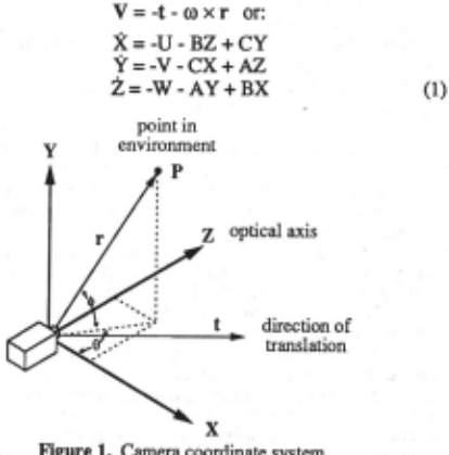
Further, we see in figure 1 that
where Lr is the length of vector r . We wish to determine the optical flow of point P in these spherical coordinates (note: it is possible to determine the optical flow for an image plane using common projection equations, however spherical coordinates are more natural for an active camera system). By differentiating the above equations, we obtain the optical flow given as:
At this point. we shall consider motion only in the X-Z plane, and not allow the camera to rotate around the X- or Z-axes. The mathematics and algorithms that follow can easily be extended to less restricted motion, but for illustrative purposes, we only consider the motion given by the vectors:
Therefore,
and thus
We now want to consider all the points that have equal flow in
the X-Z plane. If we set 6 constant and «!> equal to zero, we obtain the solutions:
where k is a constant.
These solutions are shown in figure 2. With a fixed k, the first solution is an equation for a circle in the X-Z plane. The radius of the circle is given by:
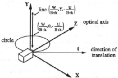
It is important to note that this circle is tangent to the camera's instantaneous translation vector. The second solution is an equation for a straight line perpendicular to the X-Z plane and intersecting the plane at the point
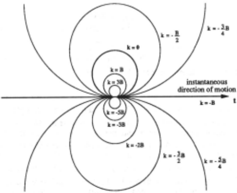
The meaning of these solutions is as follows: For a given k, all points that lie on the circle and line described in the above equations will have equivalent optical flow. Since all of the points on the circle have equivalent optical flow, we shall refer to the circle as an iso-flow circle. When we vary .k, we obtain a set of circles which all intersect at the camera's focal point, as shown in figure 3. We can consider this set of iso-flow circles as iso-flow contours. The values of optical flow corresponding to the iso-flow contours depend on the values of k, the direction of gaze, and the amount of camera rotation. However, for any direction of gaze and any rotation. the circular shape of the contours remains the same.
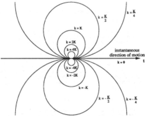
In figure 3a, we consider the case when the camera undergoes only translational motion while gazing straight ahead. We see that when k = 0, i.e., when the optical flow is zero, all of the environmental points with zero optical flow lie on a straight line pointed in the direction of motion. This is true for any gaze direction. This makes sense from an FOE standpoint, since this line will intersect the image plane at a single point, i.e., the FOE (or Focus of Contraction (FOC) if the camera is pointed backwards).
In figure 3b, the camera undergoes both translation and rotation while looking along the instantaneous direction of motion, given by the vectors t = (U,O,W) and ro = (O,B,O). We now see that all of the points with zero optical flow now lie on a circle, referred to as the Zero Flow Circle (ZFC) [11]. From this we can see that since the points on the ZFC will project onto the image plane at many different points, a single FOE point will not exist. It is also important to note that all of the points inside of the ZFC will have optical flow values opposite in sign from the optical flow values outside the ZFC. Also, points that fall on the line of instantaneous translation will have optical flow equal but opposite in sign from the rotational component of the camera.
3 Motion Parallax
Motion parallax, or sometimes called kinetic depth, is the sensation of visual depth obtained by a moving observer while fixating on a point in the visual scene. Objects in front of the fixation point move in the direction opposite of the observer movement, while objects behind the fixation point move in the same direction. The apparent velocity of each object near the fixation point is proportional to the distance from the fixation point [10]. Experiments have been carried out in the real-time computation of kinetic depth using an active camera, showing that such calculations are easy to compute when constraining the camera motion [13].
Motion parallax is easily understood when considering the iso-flow circles developed in section 2. When tracking, the fixation point must lie on a zero-flow circle that also intersects with the moving observer [11]. Objects inside this ZFC will move in the opposite direction of the observer, and objects outside of it will move in the same direction as the observer. Motion parallax will occur anytime the direction of the fixation point is not directed along the instantaneous translational vector of observer motion, i.e., when the line of sight crosses more than one iso-flow contour. This holds true when the camera undergoes any amount of rotation.
A general case of motion parallax is illustrated in figure 4. We consider the camera at two positions along a line of translation, position P1 and P2· The optical axis of the camera always intersects at the fixation point Z during motion. We also consider a point A and a point B that lie in front and behind the fixation point Z respectively. The image motion of point A is given by angle a, and of point B by angle (3. What we wish to show is how a and l3 change as the angle 6, formed by the line of sight through the fixation point and the line of translation, changes. If we define Zt and Zz as the distances from the fixation point to the robot at positions p1 and P2 respectively, then we can write Z2 in terms of Zt using the Law of Cosines:
From the Law of Sines, we know that:
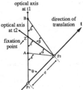
Combining these two equations, we can express angle z in terms of d, 6, and Z1:
In a similar fashion, we can determine equations for the angles a andb:
Finally, to determine a and 13, we see that:
We set the values of At. Zt. Bt. and d constant, and plot a, 13, and their difference a-13 for 6 ranging from 180° to 0°, shown in figure 5. From this we can verify that the motion parallax of points A and B given by a and 13 is zero when 6 = 0° or 180°, i.e., when the line of sight is directed along the line of translation. Further, both a and 13 go through a maximum near 90°. The functions a(6) and 13(6) act very much like the sine function, and indeed, when dis relatively small compared to At. Z1, and Bt. a(6) and 13(6) can be approximated by:
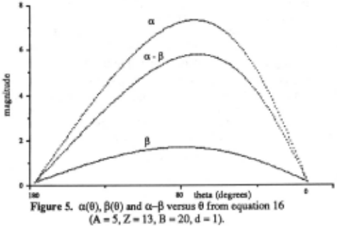
A key thing to notice in figure 5 and equations 17 and 18, is that the amplitude of a is greater than the amplitude of 13 for all values of e. That is, points nearer to the observer than the fixation point will flow in the opposite direction of the observer motion, and because they are closer, they will have greater magnitude than the flow of points behind the fixation point. Cutting suggested that humans use this information in determining the direction of motion [10]. By grouping the flow vectors moving in one direction from a group flowing in the opposite direction, and by calculating the average magnitude of flow of each group, it is possible to determine the direction of observer motion. If a group of flow vectors has greater magnitude than the other group, then the observer movement is in the direction opposite to the motion of the group of greater magnitude. However, there are cases where this concept fails. If the closer group of points are close to the fixation point, and the far group of points are far from the fixation point, then the magnitude of the closer group shall be smaller than the distant group. This problem can be rectified through an intelligent choice of fixation points. By choosing a fixation point so that there are ample scene points between the observer and fixation point, and more specifically, that there are points closer to the observer than the halfway mark to the fixation point, then the problem is eliminated.
4 Egomotion Determination Algorithm
4.1 General Strategy
In order to determine the direction and rotational component of robot motion, we use two different kinds of camera motion. We first choose a point in the environment andf'uate on it while we move a short distance. During fixation, we compute any motion parallax that occurs from points that lie on or near the line of sight. Based on the measure of motion parallax, we then saccade the camera, selecting a new view direction. A new fixation point is then selected, and the process repeats. The algorithm converges so that the camera is always pointed along the direction of instantaneous translation, where no motion parallax occurs.
The assumptions of this method are:
- The robot motion to be measured must change slowly enough so that the saccadic algorithm is allowed to converge.
- There must exist objects in the environment that are closer than half the distance between the camera and the fixation point. This insures that the average motion of objects behind the fixation point moves less than the average motion of objects in front of the fixation point (This is easily realized in the case of a mobile robot by directing the view slightly downwards. Since there are usually points seen on the ground that are much closer than a chosen fixation point, the assumption is satisfied).
The steps of the algorithm are:
- Regardless of where the camera is pointed, we choose a fixation point in the center of the field of view (In the case of a mobile robot, the camera is tilted slightly downward with respect to the mobile platform, so that the fixation point usually lies on the ground).
- The fixation point is tracked as the robot moves for a fixed distance along the path. During tracking, we measure the flow of scene points that are imaged near the vertical line passing through the fixation point. We group the flow vectors into a left-moving group and a right-moving group. We then calculate the average magnitude of flow (only in the X -direction) within each group. We call the resulting value of the left-moving group AML (Average Magnitude Left) and the value of the right-moving group AMR (Average Magnitude Right).
- A new view direction is calculated, given by:
where ei is the previous view direction, and K is a control constant that determines how quickly the the algorithm converges to choosing a fixation point along the instantaneous direction of motion. The value of K depends on the length of the tracking step, the focal length, and a limit determining how close objects may come to the camera (The choice of K is discussed later when we consider convergence and stability).
- The camera saccades to the new view direction, and the process repeats from step 1.
As the choice of fixation points approaches the line of translation, the K(AML - AMR) term in equation 19 goes to zero, and the selected view direction will converge so that the camera always points along the line of translation. While tracking fixation points that lie on the line of instantaneous translation, the tracking velocity will be equal but opposite in sign to the robot's rotational velocity. This fact is confirmed in figure 3b, where the optical flow value of the line of instantaneous translation is always -B. We thus know both the direction and rotational component of robot motion.
4.2 Convergence and Stability
Considering the AML and AMR values as single points in front and behind the fixation point, we can model the (AML - AMR) term in equation 19 simply as a - ~. where a and ~are given in equation 18. Therefore, equation 19 takes the form of:
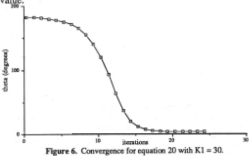
where Kt is a cumulative constant made up of the constant Kin equation 19, along with the terms A, Z, B, and d from equation 18. It can be shown that equation 20 converges to zero when K1 < 90 for all initial values of e in the range from -1t to 1t. As an example, the convergence is shown when Kt = 30 in figure
6. Note the convergence is slower when e is close to 180°. Even though at 180° the gaze direction is along the line of instantaneous translation, the algorithm will tend to diverge away from that point due to any small disturbing rotational value.
Since we do not know a priori the values A, Z, and B for each selected fixation point, we can not immediately choose an optimum constant K in equation 19 for convergence. However, we can insure convergence and stability by choosing K with knowledge of the maximum possible length of any flow vector used in determining AMI.. or AMR. Knowing the geometry of the moving platform and attached camera, it is possible to determine how close environmental objects can get to the camera. By knowing the foca1 length of the camera and the closest possible distance of an object in terms of the translational motion during the tracking period (with corresponding movement d), we can determine the maximum possible flow that object will have when imaged. We consider the extreme case when the fixation point is at infinity and we are viewing perpendicularly to the direction of motion. K then can be chosen so the saccadic algorithm will always converge:
where maxflow is the maximum largest flow of any object. K should be chosen close to this value for rapid convergence, but should remain less than the value in order to insure stability.
5 Experiments and Results
Both simulated and real world experiments were carried out to show the effectiveness of our method:
5.1 Simulation
The movement of a robot with an active camera was simulated on a Sun workstation in various environments such as a flat floor with objects, an approaching wall, and objects randomly placed in 3-D space. Both linear and curvilinear paths with different degrees of rotation were simulated. In the simulation, the focal length of the camera was set to 300 pixels and the image plane consisted of a 512 x 512 array. The robot moved in one-step units, and the camera's focal center was 2 units above the floor. In the flat floor simulation, the camera tilt angle c1> was set to a constant 11° down from the horizontal robot axis, therefore the fixation point generally was selected 10 units away. We allowed no imaged object point to come closer than 2.5 units to the robot, therefore, the maximum flow of an object point was no greater than 85 pixels. For this reason, K was chosen to be equal to one in the simulation.
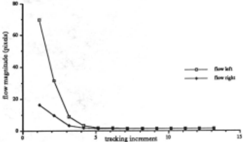
The algorithm was executed using many different rotational values, including the case of zero rotation resulting in pure translation. In all cases the algorithm converged to Within 10% of the final correct rotational value in 7 steps or less. We show the flat floor case where the robot rotates 3° counter-clockwise for each unit of forward translation in figure 7. The initial camera angle starts at 90° to the left of the direction of motion.
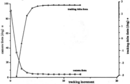
Figure 7a gives the camera angle relative to the instantaneous direction of translation after each saccadic step. We see that the algorithm rapidly converges to a final camera angle slightly less than 2°. Therefore, during the tracking step, the camera's Z axis crosses the line of translation, resulting in equal angles at the start and end of tracking. Figure 7a also shows the tracking delta theta value, which should be equal to the robot rotation component after convergence. We see that convergence occurs after 5 steps, with a fmal value of 2.9°. Figure 7b shows the values of AMI.. and AMR for each algorithm iteration. We see that the AML dominates until convergence when they are roughly equal. Figure 7c shows the simulated view from the camera with the associated motion parallax when the camera tracks at the initial angle of900.
5.2 Real-World
We have carried out the same algorithm in a real world experiment. An active camera was attached to a robot, which moved along the perimeter of a circle whose radius was 430 millimeters. The camera only rotated around theY-axis, and had a focal length of 1240 pixels. The camera was tilted down so that the ftxation points were chosen on the floor at around 1.5 meters. Objects were not allowed to come close enough to the camera so as to generate flow larger than 90 pixels. Therefore, we set K = 1 in the saccadic control equation so that the convergence of the al§orithm was guaranteed.
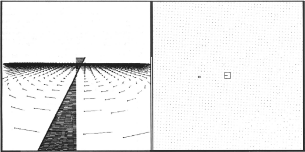
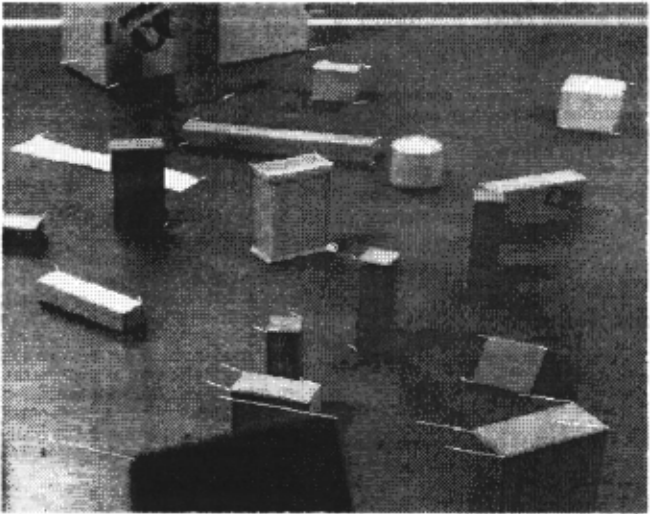
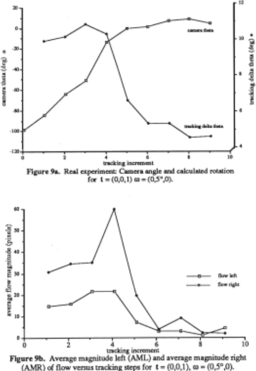
The robot moved 5 for each tracking step (38 mm translation). We had initially pointed the camera at -100° from the direction of translation. The flow of objects points near the center vertical line was measured, and AML and AMR values were determined. Figure 8 shows the scene observed during the step when the camera was oriented at -85° from the direction of translation. Also in the ftgure are the flow vectors associated with object points. The ftxation point is near the center of the image, identifted by a small circle. We see that the near objects have large flow moving right, and far objects have small flow moving left.
The results of the convergence are shown in ftgure 9. We see that the algorithm converged to a measure of robot rotation of 4.7°. The measured rotation remained within ±0.3° of this value. In ftgure 9b, we see the relative values of AML and AMR. At the fourth step, we can see that there was a very close object so as to give a high AMR value. The resulting 6% error is due to an accumulation of error in the measure of the tracking delta theta. tracking error of the fixation point, and error in the measure of the flow vectors in determining AMI.. and AMR.
6 Discussion and Conclusions
We have developed a computationally inexpensive methodology for determining robot rotation and translation by using an active camera that tracks fixation points and subsequently performs saccadic motion. Through the use of controlled saccadic motion, the rotational and translational values of motion can be determined after a few iterations of the algorithm. If the motion of the robot changes smoothly along its trajectory, the algorithm will 'track' the instantaneous direction of motion, and will provide continuous egomotion values for any type of path. It is important to note that our method simultaneously provides rotation and translation information, rather than the usual method which first determines rotation and then derotates an image in order to find the FOE and thus the direction of translation.
Note that this method does not assume that the forward pointing axis of the vehicle coincides with the instantaneous direction of motion. Such an assumption can be made for vehicles with conventional forward wheel steering with no wheel slippage. In this case, a similar but somewhat simpler algorithm can be used when the camera's rotational angle is known with respect to the forward direction of the vehicle [ 14].
We have encountered a small percentage of error in our experiments. This error could be reduced by improving the angular resolution of our active camera. Also, the algorithm depends highly on accurate tracking, so error in the tracking algorithm needs to be minimized. Accurate flow measurements are also important (albeit only near the center vertical line), so we must employ an optical flow method which is precise and robust. For speed considerations, we are currently developing a method that determines the optical flow only along the center vertical line. We intend to continue experimenting with our method, and eventually wish to perform the egomotion calculations in real-time.
@inproceedings{ijcai1991p184,
  title     = {Determining Robot Egomotion from Motion Parallax Observed by an Active Camera},
  author    = {Barth, Matthew J. and Ishiguro, Hiroshi and Tsuji, Saburo},
  booktitle = {Proceedings of the Twelfth International Joint Conference on
               Artificial Intelligence, {IJCAI-91}},
  publisher = {International Joint Conferences on Artificial Intelligence},
  editor    = {John Mylopoulos and Ray Reiter},
  pages     = {1247--1255},
  year      = {1991},
  month     = {8},
  note      = {Robotics},
  url       = {https://ijcai.org/proceedings/1991/184},
}
TY - CPAPER TI - Determining Robot Egomotion from Motion Parallax Observed by an Active Camera AU - Barth, Matthew J. AU - Ishiguro, Hiroshi AU - Tsuji, Saburo T2 - Proceedings of the Twelfth International Joint Conference on Artificial Intelligence, IJCAI-91 PB - International Joint Conferences on Artificial Intelligence PY - 1991 SP - 1247 EP - 1255 UR - https://ijcai.org/proceedings/1991/184 ER -Copied
Machine-readable versions of this paper, for tools and AI agents:





