Generating Integrated Interpretation of Partial Information Based on Distributed Qualitative Reasoning

1 Introduction

~itua~on assessment (SA), important for developing an mtel_hgent autonom~us system, is regarded as a problem solvmg_ p~ess ~ mvolves the acquiring and integrating of parual mformabon sensed from the world in order to produce a global interpretation. A notable new approach called distributed sensor network (DSN) has recently been

Osamu Katai Sosuke Iwai Tetsuo Sawaragi

Dept. of Precision Mechanics Faculty of Engineering Kyoto University Yoshida Honmachi, Sakyo-ku Kyoto 606-01 JAPAN

Hiroshi Masuiebi

FUHXERO:xe 3-3-5, Akasaka, Minato-ku Tokyo 107 JAPAN

developed. DSN consists of a number of ·sensor nodes· each of_whi~h has its ~wn knowledge or model to~ a partial mterpretation by matching the obtained information with its model. These nodes also exchange their partial interpretations with other nodes in order to integrate them into a consistent global interpretation. Researchers have tried to establish a DSN by integrating the current sensing technology with artificial intelligence methodology [Wesson et al., 1981].

In this study, we introduce a qualitative model [de Kleer, 1977] on the world into each sensor node as shown in Figurel(a). Since, in spatial and temporal terms, the sensor information obtained is local and partial for any occurring event, a qualitative model by which unknown porti?n ?f such events can be inferred should be employed; that IS, It should enable spatial and temporal interpolation to be done. Furthermore, since the sensor information involves a certain degree of uncertainty due to noise, the inference method should be robust. Taking these requirements into considcntion, we wiU introduce a qualitative model which consists of qualitative constraints derived from common sense knowledge about the sWcttite and bellavior of the world in question.

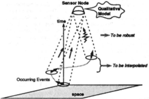
nodes and ,integrate them , fnto a global figure 1: Proposed Distributed Sensor Network with qualitative model on the world

inconsi~l~n~ · l>~anchings tp generate a consistent inte,rpretation .. froin · ampng numerous possible interpretations. · ;

Figurel(b) shows an . overview of the proposed DSN system having the qualitative model. The system consists of two types of nodes, a .sensor node and. an integration node. Since each piece of sensOr information is local and partial, w~ · can ·regard the Total World as consisting · of a certain number of Partial Worlds. To ~l;t Partial World, a sensor node is attached which ,obtains partial informatiQn concerning an event in that world, and matches the information with the model to produce a partial interpretation. In this case, the interpretation is an a posteriori evolution of that event. Due to lack of information, however, the evolution produces numerous vestigial branches. The inte_g,rat~Q9 . node(,thus functions to receive the various partial inteq>reiations from the sensor interpietation. That is, since it knows the temi>oral and spatial relationships that hold among ibe obtained· information, ttl~ node can pn'Ine the

In the ~ystem shown in IIigurel(b), the individual seqso! ~ode~ ru:e d~ti:i~uted on task lQad to reduce the whol~ .lqad of the sys~m. s!!lce these nodes share the same tasks an<;l can execute thetr tasks in parall~l,~ By contrast, the sensor node and the integration riode aie distributed qn · run~tion, 'because' these 'iwo types of nodes have dtffereri,t ~sks and''execute their tasks in parallel. ? ' '

In Section 2, we explain an architecture of the prow~. DSN system, taking an object i:noving on a slope as an" example "worfd. In Section 3: we discuss events occuqing sequ.entially in the world, and r.epresent the occurring processes as a finite state system. In the real world, howe-ver, we wm usually find that a number of events are occw:ring simultaneously. These events can not be represented by a finite state system. Thus, in Section 4, we introduce Predicate-Transition net [Reisig, 1985] as a representation method which can model concurrent events such as multiple -objects behavior on a slope. Experimental systems for the example world stated in Sections 3 and 4 are implemented by the parallel processing language, OCCAM [Pountain and May, 1988].

2 Architecture of the pr-oposed system

In order to explain the proposed system more concretely, we wiii take the e~amp~e .world of ~n.opject moving on a slope shown in Figure2(a), where the world is defined as the total slope. The sensors are initially set at some points on the world. To each sensor, a sensor riode is attached as shown in Figure2(b). Based on sensor positions, we can divide the world into Partial Worlds 1, 2, ... As shown in Figure2(b), each sensor monitors the boundary point between Partial World i-1 and i for some i. Thus when the sensor detects the partial information, Ii,j (i; sensor number, j; information number), i.e., the object crossing to the right at that point, the attached sensor node activates an interpretation process of Iij (IP-Iij). This process generates an evolution based on the qualitative model of object behavior on Partial World i (MODEL of Partial World i) to meet kinematic constraints, and sends the evolution, that is, the local interpretation of Iij. to the integration node.

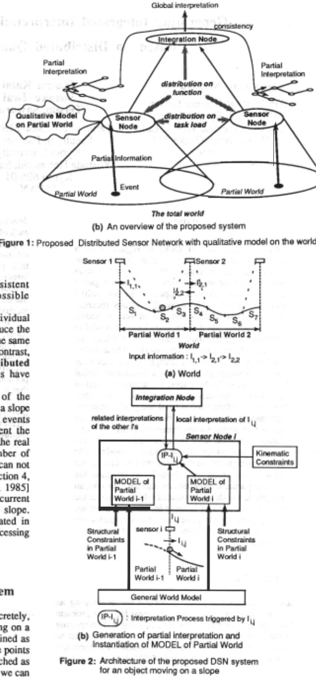
MODEL of Partial World i is an instantiation of the General World Model mentioned in the next section, which represents the object behavior on slopes of any structure. If the structural constraints of Partial World, that is, the connective relationships among St. S2, ... , are given, a General World Model is compiled and a concrete MODEL of Partial World i is instantiated.

3 Generating Interpretations of Single Object Behavior on Slopes

3.1 Snapshot discretization of a single object's continuous behavior

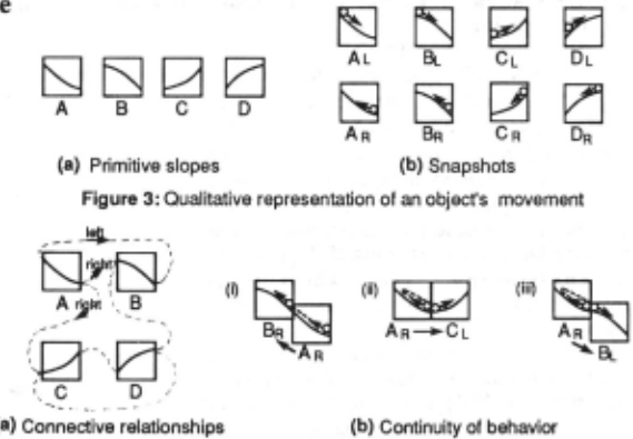
We can regard the slopes of any structure as consisting of a number of primitive slopes shown in Figure3(a), if we divide that slope according to its flexion, maximum, or minimum points. An object's behavior on these primitive slopes can be described as representations, called snapshots, shown in Figure3(b). For example, snapshot AL represents the object moving to the right from the left edge of slope A. Thus, an object moving on any slope can be represented as a connected series of these snapshots.

In connecting snapshots, we have to take into consideration the two conStraints shown in Figure4: the connectivity among the primitive slopes and the continuity of the object behavior on the connected slopes. One constraint is that, for instance, slope A's right boundary can be connected to B or C's left boundary, but not to D's, as shown in Figure4(a). As an example of the other constraint, snapshot AR can be connected to either snapshots BR, Q or BL as shown in Figure4(b). Connections (ii) and (iii) are unique qualitative representations; that is, in the usual representation, the object behavior of changing direction can be described as a series of three events; "the event of moving to the left through the right edge of slope A" -> "the event of changing its direction on the slope" -> "the event of moving to the right through that edge of A". By contrast, the representations we propose simplify this series of events by not specifying the middle event. Namely, in our method, the middle event can be interpolated by the other events. This makes our behavioral representation simpler.

3.2 Finite state diagram representation for snapshot changes

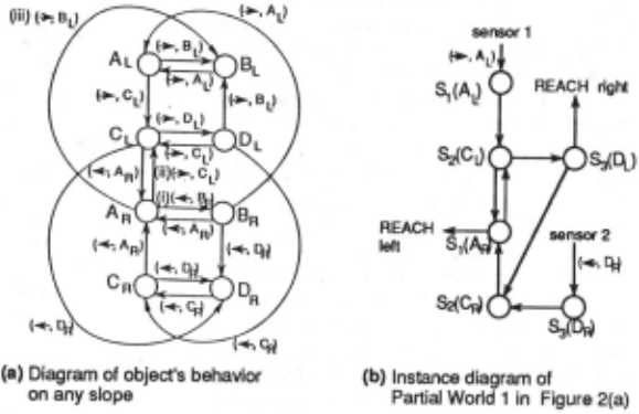
When we regard a snapshot as a state and a snapshot change as a transition, we can obtain the finite state diagram shown in Figure5(a), which is the General World Model shown in Figure2(b). This is a structural representation for object behavior on any slope, and does not depend on the concrete structure of the instance slope in question.

3.3 Concrete model of single object behavior on an instance slope

If the connective relationships of the instance slope are given, the General World Model shown in Figure5(a) is compiled and a concrete model is instantiated. For example, the relationships of the slope of Partial World 1 in Figure2 are that slope S 1 is an A-type, which is connected on the right to a C-type slope S2. Based on these relationships, an appropriate part of Figure5(a) is chosen and instantiated. Figure5(b) shows an instantiation diagram, which represents the object behavior on Partial World 1 of Figure2(a).

3.4 Kinematic constraints on single object behavior

We will now consider the following two constraints about object behavior.

Kinematic constraint 1:

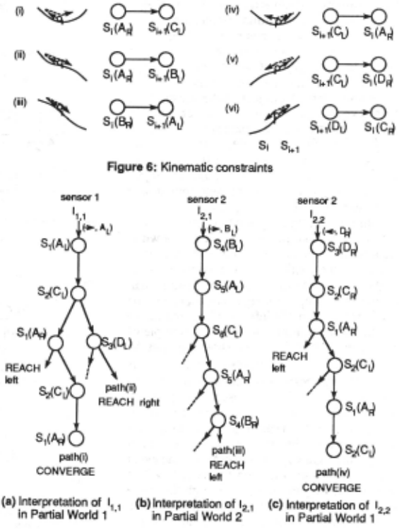
On a slope consisting of slopes Si and Si+ 1. if any one of the transitions between the two snapshots shown in Figure6 (i), (ii), ... , (vi) occurs, then whenever the object comes back to slope Si or Si+ 1 again, the same transition between snapshots will necessarily occur.

Kinematic constraint 2:

If the transitions of either (i) or (iv) occur, then the object will go back and forth around the connecting point between slopes Si and Si+1· and will "converge" on that boundary point.

3.5 Generation of partial interpretation and its integration

The Interpretation Process(IP) of sensor information (IP-Ii,j) using the model of Figure5(b) is initiated when sensor 1 gives a trigger signal activating state S 1 (AL), or sensor 2 gives another signal activating state S3(DR). After IP-Iij is started, the qualitative behavior, which is the prediction after the trigger signal, is generated by state transitions, which must meet the kinematic constraints. IP-Iij generates an envisioning tree which is an interpretation of partial information from a sensor.

Figure7 shows envisioning trees on the world, wherein (a) shows a tree which is generated by IP-I1,1· In path (i), the object converges around the connecting point between slopes S 1 and S2, since this path meets kinematic constraint 2. Path (ii) shows the object reaching the right boundary of Partial World 1. IP-I1 1 sends a tree-like structure into the integratio~ node, and IP-I2,1 and IP-I2,2 also send their structures to the same node.

In this example, the integration node receives three envisioning trees: those of I 1 1. I2,1 and I2,2· Since this node knows that Ii,1 is followed by I2,1. and that the right boundary of Partial World 1 is connected to the left boundary of Partial World 2, it selects path (ii) in Figure7(a), which describes the object reaching the right boundary of Partial World 1 as the proper interpretation. The integration node thus relates path (ii) with the tree on Partial World 2 of Figure7(b). Furthermore, since I2,1 is followed by I2,2. it selects path (iii) in Figure7(b), which describes the object changing direction on slope S6 and reaching the left boundary of Partial World 2. The integration node thus relates path (iii) with the tree of Figure7(c). In this example, since no other information is obtained after I2,2. the integration node selects only those paths in the tree (Figure7(c)) which describe the object converging around the concave point in Partial World 1, i.e., the connecting point between slopes S 1 and S2. The integration node thus generates an integrated tree-like structure consisting of path(ii) -> path(iii) -> path(iv) and so on, as the consistent interpretation of object behavior on the Total World.

4 Generating Interpretation of Multiple Objects Concurrent Behavior

4.1 General constraint about multiple objects concurrent behavior

Multiple objects behavior is regarded as an asynchronous and concurrent process subject to the following general constraint:

Two objects which are side by side move holding the relative relationships of position between them.

In other words, an object on the right side can not "go through" an object on the left side.

4.2 Representation or the constraint by Predicate/Transition net

Since an asynchronous and concurrent process such as multiple objects behavior can not be represented by a fmite state system, i.e. MODEL of Partial World in FigureS, we will introduce Predicate{fransition net (Ptr-net) [Reisig, 1985], which can precisely represent the dependency and independency of that process. Ptr-net is a high level Petri net, in which being true or not on a predicate denoted by a place depends on what "individual token" exists on that place. When the constraint on multiple objects behavior is described, each individual token denotes each object named "a", "b", and so on.

4.2.1 Predicate Place for representing the relative relationships between multiple objects

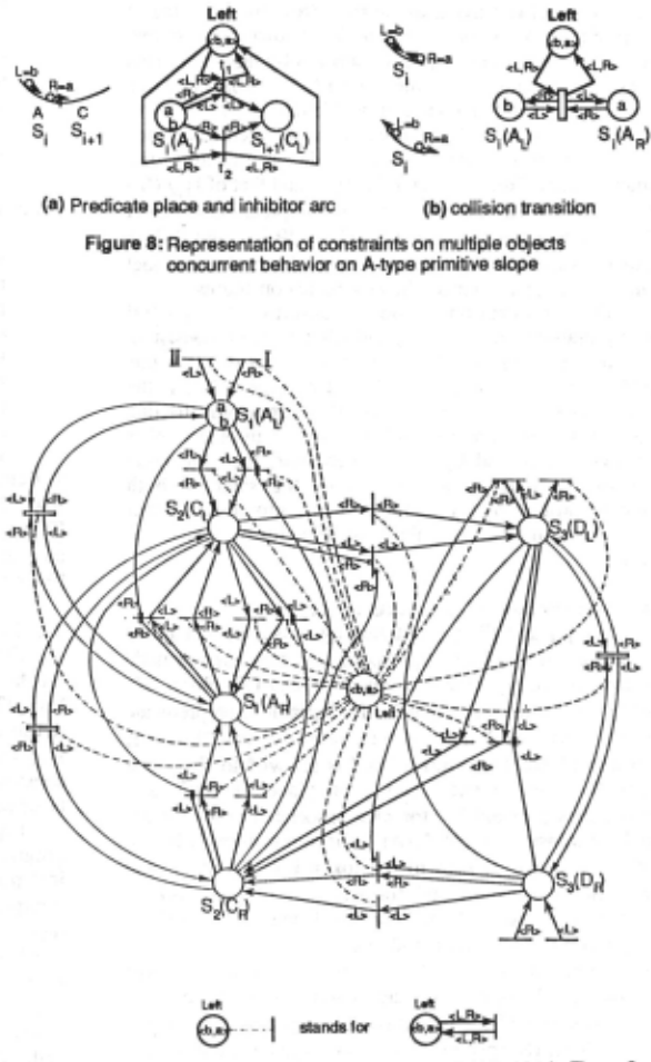
As shown in the left-hand side ofFigure8(a), the left and right objects are moving on a slope consisting of Si and Si+1· The constraint on this slope is represented in the right-hand side of that figure. Two individual tokens, a and bon place Si(AL), show that both the left object "b" and the right object "a" are moving to the right on slope Si. Place "Left" is a predicate place, which represents that variable L is to the left of v~ble R when a coupled token <L.R> exists. In Figure8(a), since object "b" is to the left of object "a", constants "b" and "a" are substituted for variables L, R, respectively. This makes Place "Left" active as shown by the <b,a> token.

4.2.2 Transition with an inhibitor arc As shown in Figure8(a), object "b" on slope S i can not move to the right slope Si + 1 without object "a" moving to slope Si+1· Arc (---o) with variable <R> linking place Si(AL) and transition t1 is an inhibitor arc, which shows that a right object moving on slope Si constrains a left object moving on that slope. That is, since predicate place "Left" is true and constant "a" is substituted for that variable R, transition t1 is not allowed to fire. By contrast, transition t2 is allowed to frre, thus token a can move to place Si+ 1 (CL).

4.2.3 Collision Transition

As shown on the left-hand side of Figure8(b), if objects "a" and "b" are moving toward one another, then the two objects will collide and move in opposite directions. This event is regarded as two changes of snapshots: change of object "b" from AL to AR, and change of object "a" from AR to AL. These two changes are represented as a transition called "collision transition" as shown on the righthand side ofFigure8(b).

4.2.4 Control of transitions by predicate place "Left"

As mentioned above, the constraint governing the relative relationships of position is explicitly represented as predicate place "Left". That is, if a sensor node acquires a piece of information concerning an object, then this node determines the name of that object, and substitutes the constant name for variables, that is, L or R of a coupled token located on that place. Thus, predicate place "Left" controls the flring of a transition with an inhibitor arc and a collision transition by substituting constants "b" or "a" for variables <L> or <R> associated with the arcs leading to those transitions.

FigureS shows the constraint on multiple objects behavior on A-type primitive slope and a slope connected to its right side. There is also the constraint on B-, C-, and D-type primitive slopes and slopes connected to both their sides.

4.3 Concrete model or multiple objects behavior

As stated in 3.3, the concrete model of single object behavior on an instance slope is generated to meet the connective relationships along that slope. A concrete model of multiple objects concurrent behavior is generated by adding the above mentioned constraint to the single object model. Thus, the multiple objects model is described as a P(f -net such as shown in Figure9, which shows two objects behavior on the slope of Partial World 1 in Figure2(a).

4.4 Generation or partial interpretation and its integration

When sensor 1 of Figure2(a) sequentially receives two pieces of information; 11,1 and I1,2. both of which mean that an object is moving to the right from the left edge of slope S 1, the associated sensor node 1 knows there are two objects, and that one object is followed by the other. This sensor node names the former object "a", and the latter one "b". Thus, since this node can decide that object "b" is to the left of object "a", the node activates predicate place "Left". Furthermore, sensor node 1 initiates the Interpretation Process of 11,1 (IP-I1,1) and that of I1,2 (IP­ I 1 ,2) ; the former generates a partial interpretation of object "a", and the latter generates that of "b". IP-11,1 and IP-11,2 execute state transition in parallel on the concrete model shown in Figure9 to meet the kinematic constraints.

The integration node integrates the partial interpretations from IP-I1,1 and IP-I1,2 into a consistent interpretation on two objects behavior. That is, since this node knows object "a" is followed by object "b", if the node finds a portion in object "a" 's behavior restricting "b" 's behavior, and also finds the portion in object "b" 's behavior restricted by "a" 's behavior, then the node determines that portion should be the same in both interpretations and integrates them into a consistent interpretation describing the total behavior of objects "a" and "b".

4.5 Generation or an occurrence net

IP-I 1, 1 and IP-I 1 ,2 initiated by sensor node 1 move tokens a and b in Figure9, respectively. Since sensor node 1 decides that I 1,1 concerns object "a" and I 1,2 object "b", IP-I1,1 substitutes constant "a" for variable Lon predicate place "Left", while IP-I 1 2 substitutes constant "b" for R on that place. Thus, tra~sition I is allowed to fire, so it actually fires to put token a on place S1(AL), and substitutes constant "a" for <R> associated with the arc linking transition I and S 1 (AL). Since transition II is also allowed to fire, it fires to put token bon S1(AL), and subs~i~utes constant "b" for <L> on the arc linking trans1Uon II and S1(AL). After this firing, IP-I1,1 and IP­ I 1 ,2 move their tokens as follows:

1. If either of the two tokens exists or both of them exist on place Si( · ), the associated Interpretation Process (IP) selects one of the transitions, ti , input place of which is Si(·). (Snapshots shown in Figure3 exist in the parentheses.)
2. It is assumed that slope Si-1 is to the left of slope Si, and slope Si+ 1 is to the right of slope Si. If the output place of ti is Si+1(·), then IP attends variable <L> on the arc leading to ti and substitutes the name of its associated token for that variable to meet predicate place "Left" supplying the constant for that variable L. On the other hand, if the output place of ti is Si-1 ( · ), then IP attends variable <R> on the arc to ti and substitutes the name of the token for the variable to meet predicate place "Left" supplying the constant for that variable R.
3. Whether ti fues or not is determined as follows:

3-1) ti is a transition with an inhibitor arc (---o).

Predicate place "Left" substitutes its constant for the variable with the inhibitor arc of ti ·. and checks whether or not the token having that constant name is located on the input place of ti. If not, since the normal arc to ti is activated by a token located on the input place of ti as mentioned in 2), ti actually fues to move that token to the output place and substitutes the name of the token for the variable with the arc to the output place. When ti is the output transition of place S3(DL), the firing of that transition distinguishes the token.

• 3-2) ti is a collision transition.

Predicate place "Left" checks whether or not the two tokens are located on the two input places as shown in Figure8(b). If one token is located on one input place linked by the input arc associated with the name of that token, and if the other token is also located on the other input place, then a collision transition fires to exchange the two tokens and to put them on the output places. Furthermore, the names of those tokens are substituted for variables with the output arcs, respectively.

4) Return to 1).

According to the above processing flow, both IP-I1 1 and IP-I1,2 generate their own occurrence nets, which de'scribe their tokens movement. These nets correspond to the tree­ like structure of state transition as shown in 3.5.

4.6 Implementation using OCCAM language

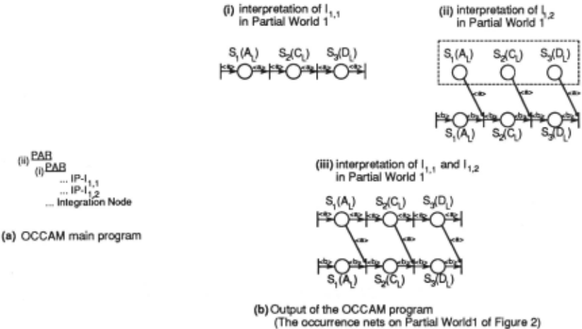
Figure10(a) illustrates an implementation by OCCAM for the inference process in the proposed system shown in Figure2. (Only the key structure of the program is shown in this figure.) PAR construction (i) declares that both IP­ I1,1 and IP-I1,2 can be executed in parallel, and PAR construction (ii) also declares that PAR (i) and Integration Node process can be executed in parallel.

Figure10(b) shows the output of the OCCAM program, that is, the occurrence net describing a piece of interpretation of I 1,1 and I 1,2· In this figure, (i) is the interpretation of 11,1 concerning Partial World 1, which represents object "a" reaching the right boundary of World 1: (ii) is the interpretation of I 1,2 representing object "b" reaching the right boundary of that world being restricted by object "a" 's behavior. Net (i) (object "a" 's behavior) is similar to the portion describing object "a" 's behavior restricting "b" 's behavior in net (ii). The integration node decides this portion to be the same among the two objects behavior. Thus, that node integrates the two interpretations into a consistent global interpretation shown in (iii), which describes that object "a" reaches the right boundary followed by "b".

5 Conclusions

In this study, qualitative reasoning techniques are introduced into the interpretation of pieces of sensor information which are local and partial from the spatial and temporal point of view. This reasoning method interpolates these pieces of information to organize them into a consistent global one. That is, thanks to the qualitative models possessed by the sensor nodes, partial interpretations of acquired information can be extended and related to each other, by which the integration node can then select the proper interpretations to generate a consistent global interpretation.

In this paper, we have taken objects moving on a slope as an example world. The sequential behavior of a single object was represented as a finite state system, and the concurrent behavior of multiple objects was represented as a Predicate-Transition net. By the use of these qualitative models, the interpolative reasoning becomes robust and is easy to implement

Acknowledgements

We are grateful to Dr. Junji Nomura, Senior Staff Researcher of Artificial Intelligence Group in Matsushita Electric Works, Ltd. for his valuable discussion and collaboration.