
A Resolution Method for Temporal Logic
Proceedings of the Twelfth International Joint Conference on Artificial Intelligence. Automated Reasoning. Pages 99-103.
© 1991 International Joint Conferences on Artificial Intelligence
Abstract
In this paper, a resolution method for propositional temporal logic is presented. Temporal formulae, incorporating both past-time and future-time temporal operators, are converted to Separated Normal Form (SNF), then both non-temporal and temporal resolution rules are applied. The resolution method is based on classical resolution, but incorporates a temporal resolution rule that can be implemented efficiently using a graph-theoretic approach.
- [Abadi and Manna, 1990] M. Abadi and Z. Manna Non- clausal Deduction in First-Order Temporal Logic. ACM Journal, 37(2):279-317, April1990.
- [Banieqbal and Barringer, 1989] B. Banieqbal and H. Bar- ringer. Temporal Logic with Fixed Points. In Proceedings of the Colloquium on Temporal Logic and Specification (LNCS Vol. 398), pages 62-74, Altrincham, U.K., 1989. Springer-Verlag.
- [Barringer et al., 1989] H. Barringer, M. Fisher, D. Gabbay, G. Gough, and R. Owens. METATEM: A Framework for Programming in Temporal Logic. In REX Workshop on Stepwise Refinement of Distributed Systems: Models, For- malisms, Correctness (LNCS Volume 430), pages 94-129, Mook, Netherlands, June 1989. Springer Verlag. 104 Automated Reasoning [del Cerro, 1984] Luis Farinas del Cerro. Resolution Modal Logics. In Proceedings of Advanced NATO Study Institute on Logics and Models for Verification and Specification of Concurrent Systems, pages 46--78, La Colle-sur-Loup, France, October 1984.
- [Enjalbert and del Cerro, 1989] P. Enjalbert and L. Farinas del Cerro. Modal Resolution in Clausal Form. Theoretical Computer Science, 65:1-33, 1989.
- [Fisher and Noel, 1990] Michael D. Fisher and Philippe A. Noel. Transformation Rules for METATEM Programs. METATEM project report, Department of Computer Sci- ence, University of Manchester, May 1990. (Draft).
- [Gabbay, 1987] D. Gabbay. Modal and Temporal Logic Pro- gramming. In A. Galton, editor, Temporal Logics and their Applications, pages 121-168. Academic Press, 1987.
- [Gabbay, 1989] D. Gabbay. Declarative Past and Imperative Future: Executable Temporal Logic for Interactive Sys- tems. In B. Banieqbal, H. Barringer, and A. Pnueli, editors, Proceedings of Colloquium on Temporal Logic in Specifi- cation (LNCS Volume 398), pages 402-450, Altrincham, U.K., 1989. Springer-Verlag.
- [Ohlbach, 1988] Hans-JUrgen Ohlbach. A Resolution Calcu- lus for Modal Logics. Lecture Notes in Computer Science, 310:500--516, May 1988. •
- Sakuragawa. 1986]
- T. Sakuragawa Temporal Prolog. Tech- nical report, Research Institute for Mathematical Sciences, Kyoto University, 1986. to appear in Computer Software.
- [Vardi and Wolper, 1986] Moshe Y. Vardi and Pierre Wolper. Automata-theoretic Techniques for Modal Logics of Pro- grams. Journal of Computer and System Sciences, 32(2):183-219, April1986.
- [Venkatesh, 1986] G. Venkatesh. A Decision Method for Temporal Logic based on Resolution. Lecture Notes in Computer Science, 206:272-289, 1986.
- [Wolper, 1982] P. Wolper. Synthesis of Communicating Pro- cesses from Temporal Logic Specifications. PhD thesis, Stanford University, 1982.
- [Wolper, 1985] Pierre Wolper. The Tableau Method for Tem- poral Logic: An overview. Logique et Analyse, 110- 111:119-136, June-Sept 1985.
References were extracted automatically from the PDF and may contain errors.
Full text extracted automatically from the PDF; figures, tables and equations may differ. The PDF is the version of record.
1 Introduction
This report describes a resolution procedure for discrete, lin ear, propositional temporal logic. This logic incorporates both past-time and future-time temporal operators and its models consist of sequences of states, each sequence having finite past and infinite future.
A naive application of the classical resolution rule to tem porallogics fails as two complementary literals may not rep resent a contradictory formula, depending on their tempo ral context. Because of such problems with resolution, the majority of the decision methods for temporal logics have been based either on tableaux or automata-theoretic tech niques [Wolper, 1985; Vardi and Wolper, 1986]. Recently, however, interest has been rekindled in the use of resolution in such logics.
The resolution method described in this report relies on a translation of temporal formulae into a normal form. This normal form is derived from that developed for use in METATEM [Barringer et al., 1989], an executable temporal logic, and the rewrite rules used to produce the normal form are derived from the work on the transformation and deter minisation of METATEM programs [Fisher and Noel, 1990]. Several of these transformations are similar to those devel oped in [Sakuragawa, 1986].
Before developing the resolution procedure in detail, an outline of the temporal logic used, will be given.
2 A Linear Temporal Logic
In this section, a propositional temporal logic based on a lin ear and discrete model of time, with finite past and infinite future, is introduced. Temporal logic can be seen as classical logic extended with various modalities. Commonly, these are (), 0, and 0. The intuitive meaning of these connectives is as follows: ()A is true now if A is true sometime in the future; OA is true now if A is true always in the future; and OA is true now if A is true at the next moment in time. Sim ilar connectives are introduced to enable reasoning about the past.
·This work was supported by ESPRIT under Basic Research Ac tion 3096 (SPEC).
2.1 Syntax
Well{ormedformulae (wft) are defined as follows.
- any element of PROP is a wff,
- if A and B are wff's, then the following are all wff's
| AvB | AAB | A=>B |
| OA | AUB | AWB |
| .A | ASB | AZB |
| OA | eA | (A) |
Further sub-classifications of temporal formulae are defined as follows. A literal is defined as either a proposition (i.e., an element of PROP), or the negation of a proposition. A State{ormula is either a literal or a boolean combination of other state-formulae.
Future-time formulae (non-strict) are defined as follows
- if A is a state-formula, then A is a future-time formula,
- if A and B are future-time formulae, then -,A, A" B, A v B, A=> B,AU B, A W B, OA. OA. and DB are all future-time formulae.
Strict past-time formulae are defined as follows
- if A and B are either state-formulae or strict past-time formulae, then OA, eB, AS B, AZ B, ~A, and .B are all strict past-time formulae,
- if A and B are strict past-time formulae, then -,A, A" B, A v B, and A=> B are all strict past-time formulae.
2.2 Semantics
The temporal logic used is based on a discrete, linear model, a, having finite past and infinite future, i.e.
Here, each Si is called a state and is a subset of PROP rep resenting the propositions that are true at the ith moment in time. An interpretation for this logic is defined as a pair (a, i), where a is the model and i the index of the state at which the temporal statement is to be interpreted.
A semantics for well-formed temporal formulae is defined as a relation between interpretations and formulae, and is de fined inductively as follows, with the (infix) semantic relation being represented by 1=. The semantics of a proposition is de fined by the valuation given to it in the model:
The semantics of the standard propositional connectives are as in classical logic, for example
The semantics of the unary future-time temporal operators is defined as follows
The two binary future-time temporal operators are interpreted as follows
If past-time temporal formulae are interpreted at a particular state, Sj, then states with indices less than i are in the past of the state Si. The semantics of unary past-time operators are given as follows:
- (a. i) 1= eA iff i = 0 or (a, i-1) I= A
- (a,i)I=OAiffi>O and (a,i-l)I=A
- (a, i) 1= ~A iff
there exists aj s.t. 0 ~j < i and (a, J) 1= A
- (a, i) 1= ·A iff for allj s.t. 0 ~j < i then (a, J) 1= A.
Note that, in contrast to the future-time operators, the + ('sometime in the past') and · ('always in the past') op erators are interpreted as being strict, i.e., the current index is not included in the definition. Also, as there is a unique start state, termed the beginning of time, two different last-time operators are used. The difference between 0 and e is that for any formula A, OA is false, while eA is true, when inter preted at the beginning of time. In particular, e false is only true when interpreted at the beginning of time; otherwise it is false.
Apart from their strictness, the binary past-time operators are similar to their future-time counterparts; their semantics is defined as follows.
(a, i) I= AS B iff there exists a k s.t. 0 ~ k < i and
(a, k) 1= Band
for allj s.t. k <j < i then (a, J) 1= A
(a, i) I= A Z B iff for all j such that 0 ~ j < i then
The 0 and 0 (and their past-time counterparts) can be de rived from the U and W operators ( S and Z) respectively as follows:
OA - trueU A
OA - A Wfalse
As an interpretation consists of a modeVstate-index pair, we say that a wff is satisfied in a particular model, at a particular state. The terminology is often extended to include a wff being satisfied in a model. A formula is satisfied in a model if it is satisfied in that model, at the beginning of time.
3 A New Approach to Temporal Resolution
When developing proof methods for non-classical logics, such as modal and temporal logics, it is natural to investi gate extending classical methods into these domains. As the classical resolution rule is of the form
one might ask whether such an inference rule can be used directly in temporal logics. Unfortunately, the use of such a rule in temporal logics has two main problems:
- Can O(A v p) and 0(8 v -,p) be resolved? If so, what is the resolvent?
This problem is characteristic of those found when res olution is required between complementary literals oc curring in different temporal contexts.
- An obvious temporal reSolution rule, extended directly from the classical rule, would be
However, sometimes the ' 0' is hidden, e.g.
This formula actually implies Op. but it is difficult to apply the resolution rule directly. Also, the resolution rule given above can not be applied to U and W for mulae.
In (2), the Op must be recognised if temporal resolution is to be applied between this formula and 0-,p. One solution to this is to provide a variety of resolution rules that 'recognise' various formulations of 0. However, as there are a large number of formulae in which' 0-like' formulae can occur, this approach is impractical.
The difficulties in recognising 0 is one of the problems caused by the interaction between the 0 and 0 operators. This interaction involves induction and accounts for many of the problems relating to the production of proof techniques for temporal logics.
The approach outlined in this report is to rewrite arbitrary temporal formulae into Separated Normal Form (SNF). The method relies on the fact that, in SNF, the only future-time temporal operator that occurs is the sometime operator, '0 '. For those literals that appear outside the scope of a 0 oper ator, non-temporal resolution is applied; for those inside the scope of a 0 operator, temporal resolution is applied.
The non-temporal resolution rule is only applied between non-temporal formulae that refer to the same state. Thus, the problem of applying classical resolution rules across temporal contexts is avoided. By the definition and derivation of SNF, any two (non-temporal) literals appearing in a formula refer to the same state.
Temporal resolution is applied to formulae containing the '0 · operator, such as (>q. In this case, the formula can be re solved with a set of formulae, s. which, when satisfied, imply that q will never be satisfied (i.e. 0--.q). As (>q guarantees that q must be satisfied at some stage in the future, the res olution rule derives the constraint that the formulae in S can never satisfied while (>q is outstanding. Thus. the second problem described above is partially solved in that once a hidden 0-formulae is found it can be resolved with a com plementary ¢-formula The actual search for the formulae that represent the 0-formula now becomes a search for for mulae on which to apply the temporal resolution rule, and this search can be implemented using graph-theoretic techniques (see §8).
The process of applying temporal and non-temporal reso lution rules to a set of formulae in SNF eventually terminates. On termination, either false has been derived. showing that the formula is unsatisfiable, or the formula is satisfiable. As in classical resolution. simplification and subsumption proce dures are applied throughout the process.
4 Separated Normal Form
Gabbay has shown [Gabbay, 1989] that for a linear temporal logic of the form described above, arbitrary formulae can be separated into their past-time. present and future-time com ponents. We use this result to develop our normal form, called Separated Normal Form (SNF).
A temporal formula in SNF is of the form
Here. each P; is a strict past-time temporal formula and each F; is a (non-strict) future-time formula. Each of the 'P; ~ F;' (called rules) is further restricted to be of one the following
where each lj. lk. or I is a literal.
Sets of rules in SNF incorporate the following restriction. For each literal, 1. there are at most two rules with a sin gle occurrence of I (i.e .· not as part of a disjunction) as their future-time component. If there are two such rules, one must be initial, while the other must be global. This ensures that there is. at most, one rule defining the initial value of I and, at most. one rule constraining I after the beginning of time.
5 Rewriting Formulae into SNF
In this section, we show how any arbitrary formula of our temporal logic can be rewritten as an equivalent formula in SNF. Rather than give the full set of transformation rules used to translate a temporal formula in this way. a few selected transformations. together with an overview of the translation process, will be presented. (A more complete description of the transformation rules will be given in the full paper - see also [Fisher and Noel, 1990] for similar rules.)
The transformation rules are given as rewrite rules over sets of formulae. In this section, we only consider the translation of formulae such as
where P; is a (strict) past-time formula and F1 is a future time formula. into SNF. The separation that was necessary to reach this form will not be considered here as it is described elsewhere [Gabbay, 1989; Barringer et al .· 1989].
The translation of the above form into SNF initially in volves removing all past-time temporal operators (apart from one level of last-time operators) from the P; and all future time operators (apart from, at most, one '0 · operator) from the F;. After these operators have been removed, the remain ing formulae must be rewritten to the correct conjunctive or disjunctive form (as described in §4).
The transformations are carried out in the context of a ' D' operator, i.e., a rewrite rule such as
is to be read as a translation from a formula such as O(A ~ B) to O((C ~D) A (E ~F)).
During the transformation process. characterised by the rewrite rules, new propositions may be introduced. These are propositions that have not previously appeared in the formula and are represented by the symbols x. y. z, etc.
5.1 Pushing Negations
Initially. some basic (simplifying) rewrites are applied. The first such set of rewrites removes D. ~.and · operators and replaces them with their definitions in terms of W , S , and Z. respectively. Next, rewrite rules that 'push' negation operators to the propositions, are applied. This ensures that all negations only appear when applied to propositions, and this translation is analogous to the translation into Negation Normal Form used in classical logics.
5.2 Removing Past-time Operators
Next. the removal of past-time operators such as S and Z , and the removal of multiple last-time operators is considered. Three (simplified) rewrite rules that are used for this purpose are given as follows 1 ·
1 Here, A ~ B is used as a shorthand for the two rules, A => B and (-,A)=> (-,B).
In the first two rules, a new proposition is introduced to rep resent the formula being replaced and its value is linked to the fixpoint representing the formula This is, effectively, the same process used in QPTL [Wolper, 1982] to represent fix point operations using quantifiers [Banieqbal and Barringer, 1989], but, because of the finite nature of the past, only one type of fixpoint is used. In the last rule, .C1 and .C2 represent arbitrary last-time operators.
5.3 Removing Future-time Operators
To remove the future-time operators, U , W , and 0, and to simplify 0-formulae so that each 0 operator is only applied to a literal, rather than a general temporal formula, the fol lowing rewrite rules are applied. Note that the :F used here represents a general future-time temporal context.
Again, the technique of introducing a new proposition symbol to represent a particular formula is used. As the 0 operator represents a maximal fixpoint, the W operator (which is also a maximal fixpoint) can be translated directly into its fixpoint definition. However, a combination of a fixpoint definition and '0' operator must be used to represent the U operator, which is a minimal fixpoint. The third rule removes all oc currences of 0 operators, and the final transformation rule is used if a 0 operator is not applied to a literal.
5.4 Rewriting Non-Temporal Formulae
Having removed all the operators that are not required in SNF, further rewrite rules can be used to translate the remaining rules into the appropriate form. This involves ensuring that all past-time components are either ·efalse' or' 0' applied to a conjunction of literals, and that all future-time components are either a disjunction ofliterals, or '0 I', where lis a literal.
As examples, we give some of the transformation rules used to manipulate last-time formulae into the appropriate form. Notice that weak last-time operators ('e ') are re moved except when applied to false.
Similar rules are used to transform future-time components into the appropriate disjunctive form.
This concludes our brief overview of the rewrite rules used for translating formulae into SNF. There are, however, some obvious simplifications that can be carried out on the rules constructed using the above rewrites. Discussion of such sim plifications will be deferred until §6.2.
Finally, note that any well-formed formula in our logic can be translated to an equivalent set of rules in SNF. As an arbi trary formula in the logic can be separated into past, present, and future components [Gabbay, 1989], the translations de scribed above can each be shown to preserve satisfiability. Though the proof of this theorem is relatively straightforwant, it does require the use of quantified propositional temporal logic [Wolper, 1982] as it must be shown that a formula in which a new proposition has been introduced is unsatisfiable if, and only if, the original formula is unsatisfiable.
6 The Resolution Procedure
Given a set of rules in SNF, both non-temporal and temporal resolution rules can be applied. Their application and effect is described in the following sections.
6.1 Non-Temporal Resolution
The non-temporal resolution rule is, essentially, the classi cal resolution rule and is only applied to 0-rules; 0-rules are processed using the temporal resolution rule described in §6.3.
The non-temporal resolution rule used here can again be expressed as a rewrite rule:
As with classical resolution, various strategies for the appli cation of this rule can be employed, and simplification rules can be used during, and after, its application.
6.2 Simplification
The basic simplification rules are
The removal of such rules is obvious, since 0 false can never be satisfied, and P ~ true is always satisfiable.
Similarly, subsumption rules may be applied. Along with the standard (classical) subsumption, the following rule for subsumption between SNF rules can be applied.
This rewrite rule can only be applied if the conditions, 1- P ~ Q and 1- G ~ F are satisfied.
If, after simplification, a formula of the form
has been derived, then the following rewrite rule can be in voked.
If this rule is used, the new constraint must be rewritten into SNF and non-temporal resolution re-applied. The process is repeated until either all 0-rules containing complementary literals have been processed, or one of the following rules has been derived.
- e false ~ false
- e true ~ false
- Otrue ~ false
If any of these formulae occur, then the original formula is unsatisfiable and the resolution process terminates.
6.3 Temporal Resolution
If the non-temporal resolution procedure described in §6.1 terminates, without false having been derived, temporal res olution can be applied.
Before applying temporal resolution, the following rewrite rule is applied to all global 0-rules. (Note that this transfor mation is not strictly necessary, but simplifies the presentation of the temporal resolution rule.)
The temporal resolution rule applies to one 0-rule, such as P ~ 0-,l and a set of global 0-rules. Here, if P is satisfied, then the rule is satisfiable unless the set of 0-rules force l to always be true. Thus, our approach is to, for every such set of rules, ensure that these, and P, are never satisfied at the same time.
The temporal resolution rule is characterised as follows.
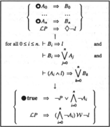
A set of rules that, together, imply that l is always true, is termed a loop in l. The side conditions on the resolution rule ensure that the the set of rules { 0Ai ~ Bi I 1 ~ i ~ n} form a loop in l. Note that even this rule is a simplification- the full rule is quite complex and does not require the application of rewrite (t) beforehand.
If a loop in l can be found, and there is a rule such as .CP ~ 0-,l, then the following new rules are added:
This rule expresses the constraint that none of the con ditions for entering a loop in l must be allowed to occur
- at the same time as P occurs.
- .CP ~ (/\7~ ..Ai) W -,l
This rule expresses the constraint that once P has oc curred, none of the conditions for entering a loop must be allowed to occur until the eventuality initiated by P has been satisfied.
6.3.1 Example
As an example, consider the set of rules representing the conjunction of the formulae described earlier, i.e.
and 0-,p. Once the formulae have been rewritten into SNF and non-temporal resolution has been attempted (none oc curs), the set of rules is as follows.
- efalse ~ X
- efalse ~ p
- efalse ~ 0-,p
5. Oy ~ pAX
Temporal resolution can be applied to rules 3, 4, and 5, as rules 4 and 5 form a loop in p. This generates the new con straint
which is rewritten in SNF as:
6. eralse ~ -,pv-,x
- efalse ~ -,p v z
11. Oz ~ -,p v z
Applying non-temporal resolution on rules 6, 1, and 2, gen erates a contradiction.
7 Correctness of the Resolution Procedure
The soundness, completeness and termination of the resolu tion procedure have been established. Proofs will be given in the full paper.
8 Implementation
Though the temporal resolution rule is complete, its use in troduces various practical problems. A naive search of all the possible subsets of rules that match the preconditions of the resolution rule would be prohibitively expensive, conse quently we have developed a procedure for finding loops in a particular literal within sets of rules. Lack of space prevents us from giving a full exposition of the approach, but we will give a brief outline below.
For every rule of the form P ~ 0-,l, all rules that imply l are collected together. This set of rules is then represented directly as an AND/OR graph, with each rule representing a set of edges, or as a standard state-graph. In either case, loops in l correspond to terminal strongly connected com ponents (SCCs) of the graph structure. These can be found through the use of a suitable version of Tarjan's algorithm. Using either representation, the complexity of the operation is exponential in the number of rules in the original set.
Once all the terminal SCCs of the graph have been found, temporal resolution can be applied to all the rules in these sees, with any new rules generated are added to the original set of rules. If no terminal sec is found, the procedure moves on to processing the next 0-rule.
9 Related Work
A great variety of resolution-based proof methods for modal logics have been developed [del Cerro, 1984; Gabbay, 1987; Ohlbach, 1988; Enjalbert and del Cerro, 1989], yet few of these can be used for temporal logics that incorporate the 'next' operator. Several resolution methods specific to tem poral logics hove been developed. Venkatesh, [Venkatesh, 1986], develops a resolution method for a future-time frag ment of propositional temporal logic using customised res olution and unwinding rules. Sakuragawa, [Sakuragawa. 1986] uses transformations similar to those described in this report to generate a normal form for temporal formulae, but does not de-..;elop specific proof rules. In [Abadi and Manna, 1990], a resolution method, based on non-clausal resolution, is developed and applied to both propositional and first-order temporal logics.
10 Further Work
A prototype system based on the approach described in this report has been implemented and initial results are encourag ing. Investigations into heuristics for the application of both temporal and non-temporal resolution rules are under way, as are investigations into alternate graph-theoretic techniques for implementing temporal resolution.
We can extend the method described in this report to first order temporal logics that have unvarying domains and that satisfy the separation property. This is current work and will form part of a future report. One point to note is that not all temporal logics allow separation, though most linear temporal logics do [Gabbay, 1989].
Finally, the resolution method described in this paper can be used as part of a backward-chaining execution mechanism that complements the forward-chaining that is standard in METATEM, a framework for executable temporal logics [Bar ringer et al., 1989].
@inproceedings{ijcai1991p15,
  title     = {A Resolution Method for Temporal Logic},
  author    = {Fisher, Michael},
  booktitle = {Proceedings of the Twelfth International Joint Conference on
               Artificial Intelligence, {IJCAI-91}},
  publisher = {International Joint Conferences on Artificial Intelligence},
  editor    = {John Mylopoulos and Ray Reiter},
  pages     = {99--103},
  year      = {1991},
  month     = {8},
  note      = {Automated Reasoning},
  url       = {https://ijcai.org/proceedings/1991/15},
}
TY - CPAPER TI - A Resolution Method for Temporal Logic AU - Fisher, Michael T2 - Proceedings of the Twelfth International Joint Conference on Artificial Intelligence, IJCAI-91 PB - International Joint Conferences on Artificial Intelligence PY - 1991 SP - 99 EP - 103 UR - https://ijcai.org/proceedings/1991/15 ER -Copied
Machine-readable versions of this paper, for tools and AI agents:





