
Learning with a Helpful Teacher
Proceedings of the Twelfth International Joint Conference on Artificial Intelligence. Learning Be Knowledge Acquisition. Pages 705-710.
© 1991 International Joint Conferences on Artificial Intelligence
Abstract
Recent work in theoretical mac,hine learning has produced many important results, primarily using the PAC-learning model. These results show algorithms to be capable of learning a concept within a certain error tolerance f: with a polynomial number of examples. Experimental machine learning, on the other hand, has produced impressive results using far fewer examples than would be required by PAClearning models. In this paper, we propose a new theoretical model in which the teacher knows the learning algorithm and chooses examples in the best way possible. We call this the Helpful Teacher model, and note that it often requires a very small number of examples to learn a concept. The model applies to both exact learning and approximate learning. We prove some lower and upper bounds for a variety of concept classes, and we observe that some of these bounds correspond closely to recent experimental results. We also note that strategies discovered using this model provide insights into the design of practical machine learning algorithms.
- D . Aha and D. Kibler . Noise-tolerant instance-based learning algorithms. In Proceeding8 of IJCAI-89, pages 794-799, Detroit, MI, 1989. Morgan Kaufmann. IJCAI
- D. Aha, D. Kibler, and M. Albert. Instance-based learn- ing algorithms. Machine Learning, 6(1), 1991.
- J. Amsterdam. Some philosophical problems with formal learning theory. In Proceeding8 of AAAI-88, pages 580- 584, Seattle, WA, 1988. Morgan Kaufmann.
- D. Angluin. Learning regular sets from queries and counter-examples. Information and Computation, 75:87-106, 1987.
- B. Baker, E. Grosse, and C. Rafferty. Nonobtuse trian- gulation of polygons . Di8crete Computational Geometry, 3:147-168, 1988.
- M. Bern and D. Eppstein. Polynomial-size nonobtuse triangulation of polygons. In Proceeding8 of the 1 g91 Conference on Computational Geometry, 1991. To ap- pear.
- W. Btintine. A critique of the valiant model. In Pro- ceeding8 of IJCAJ-8g, pages 837-842, Detroit, MI, 1989 . IJCAI
- Morgan Kaufmann.
- S. Cost and S. Salzberg. Exemplar-based learning to pre- dict protein folding. In Proceeding8 of the 1990 Sympo- 8ium on Computer Application8 in Medical Care, Wash- ington, DC, November 1990.
- S. Cost and S. Salzberg. A weighted nearest neighbor algorithm for learning with symbolic features. Technical Report JHU-90/11, Dept. of Computer Science, Johns Hopkins University, 1990.
- T. Cover and P. Hart. Nearest neighbor pattern clas- sification. IEEE 1ran8action8 on Information Theory, 13:21-27, 1967.
- S. Goldman and M. Kearns. On the complexity of teach- ing. In Proceeding8 of the 1991 Worbhop on Computa- tional Learning Theory, Los Altos, CA, 1991. Morgan Kaufmann. To appear.
- D. Haussler, M. Kearns, N. Littlestone, and M. War- muth. Equivalence of models for polynorniallearnability. In Proceeding8 of the 1988 Work8hop on Computational Learning Theory, pages 42-55, Los Altos, CA, 89. Mor- gan Kaufmann.
- D . HeliDbold, R. Sloan, and M. Warmuth. Learning nested differences of intersection closed concept classes. In Proceeding6 of the 1989 W ork6hop on Computational Learning Theory, San Mateo, CA, 1989. Morgan Kauf- mann.
- M . Kearns. The Computational Complexity of Machine Learning. PhD thesis, Aiken Computation Laboratory, Harvard University, 1989. TR-13-89.
- M . Kearns, M. Li, L . Pitt, and L. Valiant. Recent re- sults on boolean concept learning. In Proceeding6 of the 4th International Worbhop on Machine Learning, pages 337-352, Los Altos, CA, 1987. Morgan Kaufmann.
- D. Kibler and D. Aha. Comparing instance-averaging with instance-filtering learning algorithms. In Proceed- ing8 of the Third European Work6hop on Learning, pages 63-80, 1988.
- Mangasarian, R. Setiono, and W. Walberg . Pat.t.ern recognition via linear programming: Theory and appli- cation to medical diagnosis. Technical Report 878, Com- puter Sciences Dept., University of Wisconsin-Madison, September 1989.
- R. Michalski, I. Mozetic, J. Hong, and N. Lavrac. The multi-purpose incremental learning system AQ15 and its testing application to three medical domains. In Pro- ceeding6 of AAAI-86, pages 1041-1045, Los Altos, CA, 1986 . Morgan Kaufmann.
- M . Pazzani and W . Sarrett. Average case analysis of conjunctive learning algorithms . In Proceeding6 of the Worbhop on Machine Learning, pages 339-347, 1990.
- F . P. Preparata and M. I. Shamos. Computational Ge- ometry: An Introduction. Springer-Verlag, New York, 1985.
- N. Qian and T. Sejnowski. Predicting the secondary structure of globular proteins using neural network mod- els. Journal of Molecular Biology, 202:65-884, 1988.
- J . R. Quinlan. Induction of decision trees. Machine Learning, 1:81-106, 1986.
- S. Salzberg. Nested hyper-rectangles for exemplar-based learning. In K. P. Jantke, editor, Analogical and Induc- tive Inference: International Worbhop All '89, pages 184-201, Berlin, 1989. Springer-Verlag.
- S. Salzberg. A nearest hyperrectangle learning method. Machine Learning, 6:251-276, 1991.
- S. Salzberg, A. Deicher, D. Heath, and S. Kasif. Learn- ing with a helpful teacher. Technical Report 90/14, Dept. of Computer Science, Johns Hopkins University, 1990.
- G. Towell, J. Shavlik, and M. Noordewier. Refinement of approximate domain theories by knowledge-based neural networks. In Proceeding6 of the AAAI-90, pages 861- 866, Menlo Park, CA, 1990. AAAI Press.
- L. Valiant. A theory of the learnable. Communication6 of the ACM, 27:1134-1142, 1984.
- L. Valiant. Learning disjunctions of conjunctions. In Proceeding8 of IJCAI-85, pages 560-566, Los Altos, CA, 1985. Morgan Kaufmann.
- S. Weiss and I. Kapouleas. An empirical comparison of pattern recognition, neural nets, and machine learn- ing classification methods. In Proceeding6 of IJCAI-89, pages 781-787, Detroit, Ml, 1.989. IJCAI
- Morgan Kaufmann.
References were extracted automatically from the PDF and may contain errors.
Full text extracted automatically from the PDF; figures, tables and equations may differ. The PDF is the version of record.
1 Introduction
The experimental and theoretical machine learning com munities have produced numerous important results in recent years. Since Valiant's introduction of the proba bly approzimately correct (PAC) learning model [27, 28], the theory community has produced results for a wide variety of concepts. To cite just a few examples, results have been proven for intersection-closed concept classes such as rectangles [13], for general closed curves [15, 12, 14, 2], and for Boolean formulas [28]. However, if one looks at the actual numbers generated by the PAC learning bounds, the number of examples required for learning (the "sample complexity") is very large com pared to the number typically contained in an experi mental data set. Similar observations, and other crit icisms of current work in formal learning theory, have been made recently by a number of experimental ma chine learning researchers, e.g., Amsterdam [3], Buntine [7], and Pazzani and Sarrett [19]. As an example of the sample complexity produced by PAC-learning anal yses, consider an upper bound given by Aha et al. [2] for a nearest-neighbor algorithm learning closed curves: to achieve a 1% error rate for a data set with 10 variables requires approximately 2 95 examples. Obviously no real data set can contain such a large number of examples. Buntine [7] and Pazzani and Sarrett [19] have proposed average-case formal models in attempts to remove this discrepancy, with some positive results.
·This work was supported in part by the Air Force Office of Scientific Research under Grant AFOSR-89-0151.
In the experimental learning community, many im pressive results have been produced in recent years, us ing a broad range of algorithms on a variety of real world data sets. For example, machine learning pro grams have outperformed experts (or other techniques) at breast cancer prediction and prognosis [18, 23, 24, 29, 17], diagnosing thyroid disease [29], predicting pro tein secondary structure [21, 8] and classifying DNA pro moter sequences [26, 9]. In most of these cases, only a few hundred examples were available in the data set.
This discrepancy suggests the following questions:
- What is the minimum number of examples needed to learn a concept?
- What is the minimal representation for a given con cept?
- What is the most effective way to teach a concept?
- What is the effect of providing additional examples to a partially constructed representation?
To answer these and other questions, we introduce a new theoretical learning model, the Helpful Teacher. In our model, the teacher knows the learning algorithm and chooses examples in the best way possible. By "best" we mean the learning algorithm requires a minimal number of training examples to learn a concept. The teacher also knows the target concept, and is able to compute a representation of that concept in the same language used by the learner. In some instances, we have found sample complexity bounds with this model that are rel atively close to experimental results. As a result, the Helpful Teacher reduces the discrepancy between theory and practice enormously and may provide new insights for experimental machine learning research.
The Helpful Teacher model also answers some of the objections raised against theoretical analysis by the ex perimental community. Because the Helpful Teacher model provides absolute lower bounds on the number of examples required for learning (in the sense that these are best-case lower bounds), these numbers can be used to guide our data-gathering efforts; i.e., we can use lower bounds for a concept class to determine the number of examples that must be supplied to a learning algorithm. In addition, the Helpful Teacher model allows us to prove that some concept classes have exponential sample com plexity, as we show below. Because this is a best-case analysis, these classes can be considered "hard" prob lems for any learning algorithm for which such a result exists.
The Helpful Teacher model also provides insight into the complexity of student-teacher interactions for real world problems. The results presented below begin to answer an important question that has not previously been asked by the machine learning community, namely: when a teacher is trying to communicate a concept via examples (whether the student is a human or a com puter) how much information must be communicated in order to ensure that the student has an accurate model of the concept? Below we show that, for many con cepts, surprisingly little information is required. In ad dition, the study of helpful teachers produces insights into strategies for good teaching, which is an area of re s~arch not usually considered within machine learning work.
In this paper, we address the Helpful Teacher problem in the framework of geometric concept classes. We as sume that the learner is using the nearest-neighbor learn ing algorithm, and we prove lower and upper bounds on the sample complexity of a variety of geometric concept classes, including half planes, rectangles, parabolas, and general polygons. Further, we should note that learn ing algorithms using the Helpful Teacher model can, for some concept classes , produce an exact description of the concept, whereas for others, such algorithms can only provide approximations (using a specified error rate, E) .
In our framework, we can give precise answers to ques tions such as where the teacher should place prototypical examples (those in the middle of the concept) or near misses (examples near the boundary of the concept). We can also answer the question of whether a representa tion is stable; namely, whether adding new examples to a model built with a Helpful Teacher will change the rep resentation of the learned concept class. This question is indirectly related to questions such as non-monotonicity ofrepresentation, i.e., whether information that was pre viously believed to be true becomes false with additional knowledge.
We should note that in the theoretical community, An gluin [4] defined a different model of a helpful teacher, in which the learner is allowed to ask questions such as "is x a positive example?" She has produced a va riety of results for learning regular expressions and for context-free grammars. Our studies differ substantially from Angluin's work. Goldman and Kearns [11] recently developed another model of a helpful teacher where the teacher selects the best sequence of examples on-line in order to minimize the number of mistakes. Their teacher does not know the learning algorithm, but the learner is required to be consistent. They have produced inter esting results for classes such as monomials and k-term DNF.
2 Nearest-neighbor algorithms
In most of our discussions below, we use a single learn ing algorithm, the nearest-neighbor algorithm, which has been a subject of study for many years (e.g., [10]) . A number of recent experimental studies have shown that the predictive accuracy of nearest-neighbor algo rithms is comparable to that of decision ·trees, rule learning systems, and neural net algorithms [1, 16, 2, 8, 9]. In the basic algorithm, examples are vectors of numeric variables, where each example is labelled with the name of a category. Assuming that all dimensions have been normalized to the same range, distance be tween two examples with n features, z = (zt, z2, ... , zn) and y = (Yt 1 Y2 1 ··· , Yn), is simply Euclidean distance: ~( zy) = JI:7=l ( Zi - Yi )2. The basic nearest-neighbor algorithm (henceforth NN) simply stores all training in stances, and classifies each · new instance by finding the nearest example in memory.
3 Applicability of the Helpful Teacher model
One reason for choosing the nearest neighbor algorithm as our first target of study is that applying the Help ful Teacher model is relatively easy with this algorithm. The teacher simply selects examples at the best possi ble locations in feature space, and provides those exam ples to the learner. With other algorithms, particularly those that depend on the order of the inputs, finding the teacher's best strategies may be much more difficult. Consider decision tree algorithms (e.g., (22]), for exam ple: how does the teacher present examples in order to produce a particular test node in the tree? The choice of points will depend on the information measure used to construct the tree. Because the NN algorithm does not depend on the order of the inputs, the teacher is saved from having to calculate the optimal order in which to present a set of training examples.
4 Sample complexity for geometric concept learning: simple cases
Let us begin by mentioning a recent PAC-learning result due to Aha et al. [2]. First, recall that PAC-learning refers to the requirement that a learning algorithm pro duce an approximately correct model with high probabil ity [27]. In particular, a PAC algorithm has probability of 1 - b of producing a model that has an error rate no more than E. In this model, examples may be drawn at random from any distribution, as long as the training and test examples are drawn from the same distribution. Aha et al. (1991] considered the class of concepts defined by closed hyper-curves (e.g., a concept whose boundary is the union of a finite number of hyper-curves of finite length). They showed that, for algorithm NN, the num ber of instances required to PAC-learn this concept class is bounded above by (ryn/fln/r)ln(fyn/ fln / 6), where n is the number of dimensions, and f and 6 are defined as in Valiant's PAC-model. 1 Using this result, if were quire, for a particular problem domain, a 1% error rate with 99% confidence, in a 10-dimensional feature space, the upper bound for algorithm NN is approximately 2 95 examples.
Note that, although the number of examples is actu ally polynomial in the error bound, it is exponential in the dimensionality of the feature space. This property is the real cause of the extremely large estimate above. Under the helpful teacher model, some concept classes require a polynomial number of examples regardless of the number of dimensions.
4.1 Learning convex concepts
One of the simplest geometric concepts is a simple line or hyperplane, which translates into the problem of learn ing to classify correctly examples from exactly two cat egories, where those categories are separated by a line, plane, or hyperplane (depending on the number of di mensions). Although very basic, this concept has proven very useful for a large number of real data sets, and is fundamental to classification techniques such as cluster analysis.
Our first observations are extremely simple; they serve merely to illustrate the type of results we will be present ing. Proofs of the following propositions can be found in [25] .
Proposition 1. Under the helpful teacher model, ex actly 2 examples are required by algorithm NN to learn a concept defined by a hyperplane in any number of di mensiOns.
Proposition 2. If the concept boundary is a convex polytope (in 2 dimensions, a polygon) with n faces, then n + 1 examples are necessary and sufficient to learn the concept exactly.
5 Approximate learning with a helpful teacher
Since algorithm NN always partitions the feature space with lines, it cannot learn curved concept classes exactly. However, NN can approximate any such class with arbi trarily high accuracy. Thus, a natural question to ask is, using a helpful teacher, how many examples are required to approximate a concept accurately?
Because we are dealing with geometric concepts, we will use an error bound f that represents the area (or vol ume, in higher dimensional spaces) of the feature space that is misclassified. Following Kearns [14] and others, we will include in f both the area that is incorrectly classified as belonging to the concept class and the area incorrectly classified as not in the concept class.
For the sake of brevity, we will simply state one result that applies to curves and provides a clean learnability result. Suppose the concept boundary is a parabola, y = kz 2 (contained in the unit square), where the area above the parabola is classified in one category, and below the parabola in the other category. In (25], we show that sueh a coneept can be approximated with error area no greater than f with
1 For ! , 6, and -y defined as arbitrary positive numbers less than one, the instances will form an ( f, -y )-net with confidence (1 - 6) . For details see [2].
points using a Helpful Teacher. In addition, we show that the strategy we have devised is optimal; i.e., for a fixed number of examples n, it minimizes the error area.
For comparison, consider the number of points n re quired under the PAC-learning model for the same con cept. (Although this example may be a bit artificial, it illustrates the difference between PAC-learning and Helpful Teacher results.) For the parabola y = z 2 , using the results of Aha et al. [2], if we set f = "Y = 6 = .001, then we haven~ 4.3 x 10 10 . Contrast this with the help ful teacher model, where with f = .001, we only need 9 examples!
6 Learning complex geometric concepts
In this section, we consider the sample complexity of learning a number of more complex geometric concepts. By virtue of their complexity, these objects have the abil ity to approximate many real-world concepts, including those with very complex boundaries. Interestingly, some of these concept classes may require a large number of ex amples, even with a helpful teacher. Unless other learn ing algorithms (besides NN) turn out to be significantly more powerful, these concept classes will remain "hard" for learning.
We first need to make some observations about learn ing triangles with the nearest-neighbor algorithm. These observations will be useful in the proofs below. First re call the definition of a Voronoi diagram: given a set of points S in Euclidean space, each point Pi has a Voronoi polygon around it that contains all points closer to Pi than to any other point. The union of all the Voronoi polygon boundaries is the Voronoi diagram of S. The partitioning induced by the NN algorithm is, by defini tion, a Voronoi diagram [20].
Proposition 3. For the concept class containing tri angulations of the plane in which all triangles are right or acute triangles, a Helpful Teacher can simply give the learner points placed around every vertex of every trian gle. The strategy is simple: for every edge, place a pair of points symmetrically on either side of the edge, arbi trarily close to the endpoints. This requires four points per edge, and if the triangulation contains n vertices, this strategy requires O(n) examples.
The Voronoi diagram produced by these points will include all edges of the triangulation, as long as all an gles are non-obtuse and as long as the boundary of the triangulation is convex. This strategy also applies to d dimensional objects in which all angles between faces are less than or equal to 90°.
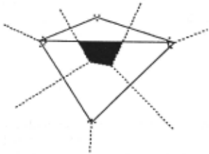
Note that Proposition 3 does not hold for obtuse tri angles. Consider Figure 1, in which an obtuse triangle is shown attached to an acute one. If the training examples are placed around each vertex, then the Voronoi diagram created will not correctly demarcate the edge shared by the triangles. Part of the Voronoi diagram is shown as dotted lines in the figure, and the resulting mis-classified area is shaded.
6.1 Rectilinear solids
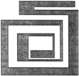
Consider the set of concepts defined by non-convex simple polygons (i.e., polygons that are not self intersecting) . Because the Helpful Teacher algorithm for learning this concept class is rather complex, we will first consider learning a subclass. Rectilinear polygon$ are polygons in which all the sides are parallel to the axes. Figure 2 shows a rectilinear polygon in two di mensions. Rectilinear concepts play an important role in our analysis because they can be used to approximate more general geometric concept classes with arbitrary precision.
Theorem 1 Any rectilinear polygon with n edges in two dimen3ion3 can be learned by a Helpful Teacher with 0( n 2 ) ezample3.
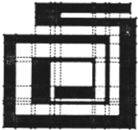
Proof. Draw the smallest possible rectangle around the rectilinear polygon. For each edge of the polygon, extend the edge in both directions until it meets the containing rectangle. The resulting grid will contain at most O(n 2 ) vertices. We can now place 4 points sym metrically around each edge coming out of a vertex, arbitrarily close to the vertex. This set of point.s will define a Voronoi diagram that contains the grid, and therefore contains the rectilinear polygon. With appropriate la belling of points, the learning is complete, having used O(n 2 ) examples. Figure 3 illustrates the grid and the placement of points for the rectilinear polygon from Fig ure 2. For visual clarity, a single dot appears in the figure at every vertex around which points need to be placed. Note that points only need to be placed around grid ver tices where the grid coincides with one of the vertices or edges of the original polygon. 0
Suppose next that we wish to learn a concept defined by an arbitrary partitioning of the plane into polygons; for example, a triangulation of the plane. For such a con cept, we may wish to allow each region of the partition ing to have a different class label. Despite the apparent complexity of this concept class, we can approzimate it using the rectilinear concepts just described.
Corollary 1.1 Any polygonal teuelation in the unit 3quare can be learned by algorithm NN with error area f, u3ing only O(n 2 /f) poinb, where n is the number of edge3 in the teuelation.
The full proof of this corollary is contained in [25) . It also extends to higher dimensions, where the sam ple complexity is O(dn 4 jfd-l ), and f represents the er ror volume. An interesting feature of our approximation technique, which involves overlaying a grid on the tes selation, is that any point that is classified incorrectly using this technique is within a very small distance from an edge of the original tesselation.
For rectilinear concepts, we also have a lower bound on the sample complexity.
Theorem 2 At lea3t n 2 /32 ezample3 are required for learning 3ome rectilinear polygon$ with a helpful teacher, where n is the number of 3ide3 of the polygon.
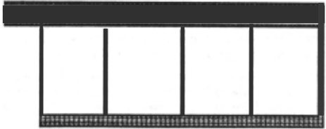
Proof. We prove this theorem by constructing a rec tilinear object that requires n 2 /32 points to define it. See Figure 4 for an example of such an object. 2 The object shown has approximately n/8 vertical "fingers" and n/8 horizontal "fingers" (since each finger uses four sides of the polygon). These fingers can be made arbi trarily thin and arbitrarily long. By placing the verti cal fingers far apart, as we have illustrated in the fig ure, we make it impossible to define the topmost (hori zontal) edge of each finger without interfering with all of the horizontal fingers. Thus a point placed above the topmost ecfge of each vertical finger will propagate through all of the horizontal fingers, requiring us to draw a pair of points around each of the edges above it. There are n/4 such edges in the n/8 horizontal fingers, which means that each vertical finger will re quire at least n/4 new points for learning (some of the points used to define horizontal edges may be shared). Therefore the total number of points required is at least (n/8)(n/4) +constant = n 2 /32 +constant. 0
2 The idea of this construction was proposed by Michael Goodrich.
The theorems for rectilinear objects given above both extend quite straightforwardly into d dimensions. Let a rectilinear polytope be a d-dimensional object for which every face (or facet) of the object is parallel to one of the axes.
Corollary 2.1 No more than 2nd examples are required for learning rectilinear polytopes with n faces (or facets) in d dimensions.
Corollary 2.2 At least 0( (~)d) examples are required to learn a rectilinear polytope with n faces in d dimen swns.
For proofs of these two corollaries, see [25].
6.2 Learning general polygons
The class of simple non-convex polygons is much harder to learn than rectilinear polygons. Because we can al ways triangulate a polygon by adding a linear number of sides, we can solve the learning problem for general poly gons by learning triangulations instead. Proving that non-convex polygons are as hard as triangulations is an open problem.
6.2.1 Triangulations of the plane
We now turn to the concept class defined by triangu lations of the plane. The learning problem here is essen tially equivalent to a current open problem in computa tional geometry. Since nearest neighbor partitions are by definition Voronoi diagrams, we can state our learn ing problem as follows: given a triangulation, what is the smallest Voronoi diagram that contains the triangu lation as a subgraph? If we find the Voronoi diagram, we have also found the points that the Helpful Teacher should use.
Our best current result for learning triangulations with a helpful teacher requires a number of points that is proportional to the largest aspect ratio (the ratio of the longest edge to the height) of any triangle.
First, recall our earlier proposition, that if all tri angles are acute, algorithm NN with a helpful teacher can learn a triangulation with O(n) examples (assuming the triangulation has a convex boundary). The problem of triangulating polygons with non-obtuse triangles has until very recently been an open problem in computa tional geometry. Baker et al. [5] produced the first so lution, which used a relatively large number of triangles (the precise bound was not given). Bern and Eppstein [6] have recently reported a solution in two dimensions that uses O(n 2 ) triangles for an n-sided polygon. Their method makes significant progress towards solving the Helpful Teacher problem, although a complete solution requires triangulating the inside and outside of a poly gon.
Theorem 3 Any triangulation of the plane can be learned with 0( f) points using a helpful teacher, where L is the total length of all edges of the triangulation, and h is the height of the shortest triangle (i.e., the triangle with the smallest altitude).
Note that even if all edges are very long, h might be extremely small if the triangulation contains very long, narrow triangles.
Proof sketch. For details see [25]. We give an algo rithm that uses 0( f) points to define any triangulation. Beginning simultaneously at both ends of every edge in the triangulation, place a pair of points symmetrically on either side of the edge, very close to the edge itself and to each end of the edge. (The distance between each point and the edge needs to be much less than h to guarantee that the resulting Voronoi diagram will con tain the edge.) Next, moving from the ends towards the middle of each edge, place a pair of points at intervals of length h symmetrically on either side of the edges. Stop when the midpoint of the edge is reached. The points placed near the midpoint may be closer together than h. If the pairs of points placed near the midpoint are at a distance greater than h from each other, place one more pair of points around the midpoint itself. The placement of points is illustrated in Figure 5. For a proof that this strategy correctly defines every edge of the triangulation, see [25].
For most triangulations, L/h is small, but assuming fi nite precision on the input, it can be exponentially large (and if one allows infinite precision, L/h is unbounded). To handle such cases, we have devised a strategy for ap proximating triangulations, presented in Corollary 1.1 above. If an area no larger than f is allowed to be mis classified, this strategy requires O(n 2 /e) examples, re gardless of the ratio L /h.

| Concept boundary | Lower Bound | Upper Bound |
|---|---|---|
| hyperplane | 2 | 2 |
| n-face convex polytope | n+l | n+l |
| parabola y = kz 2 , £error area | ftA+ll | ftA + 1 1 |
| Acute/right n-triangulation | O(n) | O(n) |
| n-sided, d-dim rectilinear polytope | O((~)d) | O(nd) |
| d-dim triangulation, Total face area A, min altitude h | - | O((~)d-1) |
| Polygonal tesselation, d-dim, n faces, £ error volume | - | d 0(.~':.) |
Corollary 3.1 In d dimensions, a modification of the algorithm in Theorem 3 suffices to define a simplicial decomposition (a multi-dimensional triangulation}. If A is the total area of all faces of the decomposition, then the number of ezamples required in d dimensions is O((A/h)d-t).
For details see [25].
7 Conclusion
The results presented in this paper show that, for a given algorithm, it is possible to demonstrate lower and upper bounds for many different concept classes using the "best case" model that we call a Helpful Teacher. Our results are summarized in Table 1. These bounds are useful for a variety of reasons. First of all, the lower bounds provide an absolute limit on the number of examples required for learning. This limit tells us in advance how many examples must be provided if we expect our algorithm to learn a concept.
Limits derived using the Helpful Teacher model may provide an instructive basis for comparison between learning algorithms. We now have theoretical models giving worst-case (e.g., [27]), average-case (e.g., [19]), and best-case analyses. Although the Helpful Teacher studies described here involve only the nearest neighbor algorithm, this is only a first step. Our next step will be to find Helpful Teacher bounds for other algorithms, such as decision trees and neural nets. In addition, we would like to consider Helpful Teacher strategies for non geometric concepts such as Boolean formulas.
Some concept classes appear to be "hard" for the near est neighbor algorithm, in that the number of exam ples required for learning, even in the Helpful Teacher paradigm, is exponential in the number of dimensions d. In particular, the class of non-convex simple poly gons (and polytopes) behaves this way. We have shown (by construction) a lower bound on a special subclass of non-convex polygons - rectilinear polygons - that ex hibits this exponential behavior. This result points out a weakness in the nearest neighbor algorithm itself; thus, if another learning algorithm can be shown to learn this class more efficiently, that algorithm could justifiably be described as more powerful than the NN algorithm.
Note that in the context of NN the minimal number of examples is equal to the size of the minimal representa tion. For other learning methods, providing the minimal number of examples does not always generate the mini mal representation. For example, a strategy to produce the minimal size decision tree for an algorithm such as ID3 may require more examples than some other strat egy that also learns a concept correctly. Although the issue of minimal representations is certainly related to our model, our main interest is in determining the mini mal number of examples and in strategies for generating these examples.
We should also take note of the following counter intuitive result: it is sometimes the case that provid ing more examples to an algorithm reduces its accuracy. This is a partial answer to the question we asked at the beginning of this paper, namely, what is the effect on a learned concept of providing the learner with additional examples? With nearest neighbor, a simple example of this effect occurs for learning a plane (hyperplane). Only two examples need to be provided; however, if one pro vides additional examples, the concept definition is likely to shift so that it is no longer accurate. This result con tradicts the prevailing wisdom that larger data sets pro duce more accurate models.
Finally, many of the sample complexity bounds given above are quite small, and in this respect they are similar to the size of real data sets used for experimental work in inductive learning. Because the data sets used for exper iments are limited in size, there is a need for theoretical results on how much learning is possible with small data sets. The Helpful Teacher model provides such results. We are currently developing nearest neighbor algorithms that discard examples in an attempt to converge to a set that is roughly the size of the bound provided by the Helpful Teacher model. We use a strategy of retaining examples close to the boundaries, inspired by our al gorithm for learning triangulations. In this work, the theoretical model is directly relevant to the design of an experimental algorithm.
Acknowledgements
Thanks to Michael Goodrich, John Johnstone, and Gre gory Sullivan for many insightful comments and discus sions on the ideas presented in this paper.
@inproceedings{ijcai1991p103,
  title     = {Learning with a Helpful Teacher},
  author    = {Salzberg, Steven and Delcher, Arthur L. and Heath, David G. and Kasif, Simon},
  booktitle = {Proceedings of the Twelfth International Joint Conference on
               Artificial Intelligence, {IJCAI-91}},
  publisher = {International Joint Conferences on Artificial Intelligence},
  editor    = {John Mylopoulos and Ray Reiter},
  pages     = {705--710},
  year      = {1991},
  month     = {8},
  note      = {Learning Be Knowledge Acquisition},
  url       = {https://ijcai.org/proceedings/1991/103},
}
TY - CPAPER TI - Learning with a Helpful Teacher AU - Salzberg, Steven AU - Delcher, Arthur L. AU - Heath, David G. AU - Kasif, Simon T2 - Proceedings of the Twelfth International Joint Conference on Artificial Intelligence, IJCAI-91 PB - International Joint Conferences on Artificial Intelligence PY - 1991 SP - 705 EP - 710 UR - https://ijcai.org/proceedings/1991/103 ER -Copied
Machine-readable versions of this paper, for tools and AI agents:





