A Critique of the Valiant Model

1 Introduction

The field of machine learning has accrued experience across a broad number of areas, and there is now a push for developing a more formal theory of learning. While we are still a long way from this general aim, funda­ mental principles exist on which such a theory should be based: statistics, the representation and utility of knowl­ edge, computational complexity [Valiant, 1985], man­ machine interaction [Bun t ine and Stirling, to appear], and the psychology of learning. Perhaps the first at­ tempt to encompass some of this broad spectrum in a formal theory was made by Valiant in his "theory of the learnable" [Valiant, 1985]; Valiant argued that a theory of learning should show classes of concepts are le,lrnable in the context of an appropriate information gathering mechanism and in a reasonable number of steps. The best known instance is Valiant's model for learning logi­ cal concepts from random examples. I shall refer to this as the Valiant model, which is distinct from his general framework. The Valiant model has subsequently been developed by a number of researchers to yield an impres­ sive array of results and research tools [Haussler, 1988, Rivest, 1987]. The Valiant model has also recently re­ ceived strong criticism from Amsterdam [Amsterdam, 1988a], who said Valiant 's formal model of concept learning ... has rarely been used in practice, in part be­ cause the known learnable concept classes are too restricted.

Amsterdam suggested a number of extensions to the model, incorporating queries and learning approximate representations of a concept, and criticised the model for its restricted scope [Amsterdam, 1988b].

The Valiant model is becoming recognised as a stan­ dard for formal learning theory and several extensions exist [Angluin and Laird, 1988, Amsterdam, 1988a, Rivest and Sloan, 1988]. But if it is to be a standard, we should heed Amsterdam's criticisms and first consider just how well the Valiant model handles its intended task, without extensions and considering only its (admittedly restricted) current scope. This paper does just that; the paper is a critique of the statistical component of the Valiant model.

The two principle claims of this paper are that the current interpretation of the Valiant model can produce overly-conservative estimates of error (even accounting for the approximations used); and that the model fails to match the induction process as it is often implemented. It is argued that these supposed shortcomings occur be­ cause the model gives sample independent bounds, the model is based on worst case analyses, and the model fails to accommodate preferences (or hunches) about hypotheses. Overly-conservative estimates would cause problems in the knowledge acquisition context, for in­ stance, where only a limited sample may be avai lable, extra examples costly to obtain, and realistic estimates of error are required regardless.

These shortcomings suggest that the statistical com­ ponent of the model is inadequate for a comprehen­ sive analysis of the problem of designing learning algo­ rithms, although the model does produce valuable up­ per bounds on learning performance . The shortcomings may be viewed as symptomatic of the underlying pseudo­ classical statistical philosophy of the Valiant model. The Bayesian approach is instead adopted here. The main theoretical machinery that this approach adds is the no­ tion of a prior. While priors certainly have to be used with caution [Berger , 1985, p109], there use allows a much more powerful statistical analysis of the logical in­ duction problem that still shares all the "distribution­ free" advantages of the Valiant model [Haussler, 1988, p179], albeit in an average-case rather than worst-case sense.

Other support for the Bayesian approach appears sub­ stantial. There are strong foundational arguments for the approach as a method of reasoning about uncer­ tainty (concept learning is an instance of such reasoning) [Berger, 1985, Horvitz et al., 1986], and the approach tackles a broad range of other problems in intelligent sys­ tems (Pearl, 1988). More relevant to the present topic, however, the Bayesian approach handles the problem of learning uncertain concepts, a central problem that the Valiant model has been criticised for not handling [Ams­ terdam, 1988b]. Bayesian methods are competitive with some other machine learning approaches [Cheeseman et al., 1988, Buntine, 1989c] . A version of Quinlan's infor­ mation theoretic heuristic for greedily building decision trees [Quinlan, 1986] can be derived from Bayesian prin­ ciples, and the widely reported tradeoff between concept simplicity and prediction accuracy has a well known ex­ planation in Bayesian decision theory [Cheeseman, 1987, Buntine, 1989a]. These last two issues have recently been reported as open problems [Haussler, 1988, Fisher and Schlimmer, 1988]. The Bayesian approach, however, only addresses the uncertainty in learning, and clearly needs to be complemented, for instance, with the com­ putational concerns that are central to Valiant's broad learning framework, and indeed crucial to any theory of machine learning.

Sections 2 and 3 introduce the task of learning logic concepts from random examples and the Valiant model to that task, Sections 4, 5 and 6 each illustrate a problem with the model. Section 7 then outlines the Bayesian so­ lution and Section 8 concludes with some open problems.

2 The learning task

The Valiant model is primarily concerned with the logic induction problem. For example, suppose for discussion that we are designing a system to plan the routing of sheet steel through a large manufacturing plant. For the purposes of deciding whether to use the annealing process or not, a product may be classified by a number of attributes that together uniquely determine whether the process should be used. That is, there is known to exist a necessary and sufficient (logical) definition of the "annealing" class given in terms of attributes, this is the classification rule we hope to approximate.

Let us assume there are 6 binary-valued attributes: cold-rolled, aluminium-killed, deep-drawing, skin-passed, exposed-surface and carbon. And we have been provided with some examples (each gives values for the attributes) that have also been classified as either positive or nega­ tive (use annealing, or not) by the resident metallurgist. In this instance, there are 2 6 = 64 possible examples, each having one of 2 possible classifications. A distri­ bution on the examples gives the frequency of any par­ ticular steel product (as uniquely determined by the 6 attributes) would occur, irrespective of its actual classi­ fication. Examples are known to have come from a fixed distribution. A random sample is a set of classified ex­ amples drawn independently and identically according to the distribution on examples. This implies sampling with replacement.

A simplistic notion of the logic induction problem, then, is to find the "true" classification rule given only the classified examples. In practice, of course, we would at best hope to find a classification rule that minimises errors in some sense on future predictions. An hypothe­ sis space 1{ represents a space of classification rules that can feasibly contain the "true" one. For instance, in the steel routing application, if we consider the complete hy­ pothesis space, all possible classification rules over the 64 examples, the space is of size 2 64 or approximately 1 billion.

3 The Valiant model

Angluin and Laird precis the statistical component of the Valiant model as follows [Angluin and Laird, 1988]:

The idea is that after randomly sampling (clas­ sified examples) of a concept, an identifica­ tion procedure should conjecture a concept that with "high probability" is "not too different" from the correct concept.

Angluin and Laird have termed this notion probably ap­ proximately correct (PAC) and a common interpretation [Haussler, 1988] is, in a nutshell: there are so few hy­ potheses left that are consistent with the classified ex­ amples that every consistent hypothesis is with a confi­ dence of 1 - 6 approximately correct with error at most f on future samples. I shall refer to this as the classical interpretation.

With 11-ll hypotheses, Blumer, Ehrenfuecht, Haussler and Warmuth lBlumer eta/., 1987) show that to be as­ sured ofPACness with error f and confidence 1-8 with a random sample of size N examples, the following should hold

I shall refer to this as the Blumer bound. For a complete propositional hypothesis space 1l over n propositional symbols, 11-ll is 2 2 n (there are 2" different examples, each can be true or false). For various other proposi­ tional languages the Blumer bound gives tighter results than those obtained using the Vapnik-Chervonenski di­ mension [Buntine, 1989b, Haussler, 1988] . For learning then, after setting an acceptable level of confidence and error, we select a plausible hypothesis space, choose an algorithm and buy the sufficient sample, and then apply the algorithm to find a hypothesis consistent with the sample.

4 The impact of the sample on estimating PACness

The classical interpretation ignores what is perhaps the most vital piece .of information in the whole equation: what actual examples are obtained. Results are always given purely in terms of the size of the sample. While this is acceptable if we currently wish to estimate how large a sample should be obtained, if we actually have a sample there may well be other information in it apart from its size able to tighten the bounds on PACness. A learning algorithm should make use of this sort of information.

To understand the potential of this other information, consider the analytically simple but impractical situation where the the hypotheses space is complete, it includes all possible classification rules. For instance, in the steel routing example, 11ll = 2 64 . With a sample of size 200 and confidence of 90% the Blumer bound gives a bound off < 0.23. Experience with induction tools such as ID3 [Quinlan, 1986] indicates that this bound is not optimal. In fact, stochastic simulation shows that according to most distributions on examples, given a random sample of 200 classified examples, many of the 64 possible differ­ ent examples will have been included, so we know their classification! Of the remaining, because we haven't seen them in a rather large sample, they are probably rare anyway. It is possible but very unlikely that the ran­ dom sample will contain all possible examples, then the predicted error rate should be zero! If only 4 out of the 64 where not included, then the error rate should now be non-zero and of the order of 4/64 = 0.0625, certainly much less than 0.23. At the other extreme, if the random sample consisted of 200 repetitions of the same example, then the predicted error rate should be higher again. Knowledge of the actual sample clearly has potential for improving error analysis, and a theory of learning should account for this.

A careful inspection of the proof of the Blumer bound reveals that it assumes the size of the sample is known, but the examples making up the sample are unknown. Information about the sample cannot be incorporated. Fortunately, a sample-dependent bound for determining PACness can be found using Bayesian statistics. This is based around a notion of the disagreement between consistent hypotheses.

Definition 1 Let S be a random sample of classified ex­ amples of a concept drawn from a finite example space and let 1i be a hypothesis space for the concept. The maximum disagreement induced by S on 1{ is the maxi­ mum for I such that H1, H2 E 1i, H1 and H2 are consis­ tent with S, and H 1 and H 2 disagree on I classifications out of all possible distinct examples.

For a complete hypothesis space, the maximum dis­ agreement induced by S is just the number of distinct possible examples that do not occur in S. For a con­ junctive hypothesis space, maximum disagreement h~ an upper bound of 2n+l-·c(S) - 2n+1-lc(S) where n IS the number of propositional symbols, sc(S) denotes the length of the shortest conjunction consistent with S, and lc(S) denotes the length of the longest such conjunction [Buntine, 1989b]. For this last bound, bare in mind that there are 2n distinct possible examples.

Disagreement can be used to find an upper confidence limit on the chance that any consistent hypothesis will disagree on the classification of an example. The result assumes the so called non-informative Dirichlet prior on a distribution over n example types, Pr(e1 , ... ,en) <X f1; e"- 1 , where e; is the probability of seeing the i-th example and a is set to ~· As always, the choice of prior is application specific so some other value of a might be more appropriate for a given problem.

Lemma 1 ([Buntine, 1989b]) Let S be a random sample of N classified examples, 1l be a hypotheses space onE distinct examples, and k be the maximum disagree­ ment induced by S on 1l. In addition, suppose that a prior belief in the distribution on examples zs non­ informative. Define beta error to be the value off for

where I, is the incomplete beta function [Abramowitz and Stegun, 1972]. For any arbitrary hypothesis H con­ sistent with the sampleS, we have better than 1-8 confi­ dence according to a posterior belief (conditioned on the sample) that the error rate of H is less than the beta error.

Fast formulae for computing the incomplete beta func­ tion and its inverse are available in mathematical hand­ books [Abramowitz and Stegun, 1972]. To give an idea of the behaviour of beta error, the following approximation can be made [Buntine, 1989b].

where Z 1_ 6 denotes the standard normal deviate for 18, that is Pr(Z < Z1_6) = 1- 8. For instance, Zo.95 = 1.64 and Zo.99 = 2.33. This approximation should be compared with the Blumer bound. Notice that k/2 and In 11ll roughly correspond in the two bounds.

Consider, again, the simple situation where the hy­ pothesis space is complete. Figure 1 shows how the beta error in which we have 99% confidence varies as a larger sample is taken. Twenty-four samples were gen­ erated by first randomly generating (according to the non-informative prior) a distribution if on the E = 64 distinct examples, and then randomly generating exam­ ples from this distribution. Two representative samples where then selected for display. Accumulated sample size is given by N. The line graphs marked by boxes and the left axis give beta error. The line graphs marked by circles and the left axis give the true value of the max­ imum error for a consistent hypothesis. Notice how the beta error usually tracks along but just above the true maximum error. This occurred in all twenty-four sam­ ples, with the beta error occasionally under-estimating error. The Blumer bound 1 is the line marked by dia­ monds in the top part of the graph. The bar graphs and left axis give the maximum disagreement induced by the accumulated sample (k) represented as a proportion of the distinct examples (k/ E). Notice how the beta er­ ror stays well below this proportion as Equation (2) in­ dicates, but the Blumer bound remains with it. With the well behaved nature of the beta distribution, similar shaped graphs should occur for other values of E and 8.

Figure 2 shows how the beta error in which we have 99% confidence varies with k, the maximum disagree­ ment induced by a sample on a hypotheses space. This is given for two different sample sizes (N = 100, 200)

1 For a fairer comparison, a tighter version 6 < IHI(l- c)N has been used in this and later graphs.

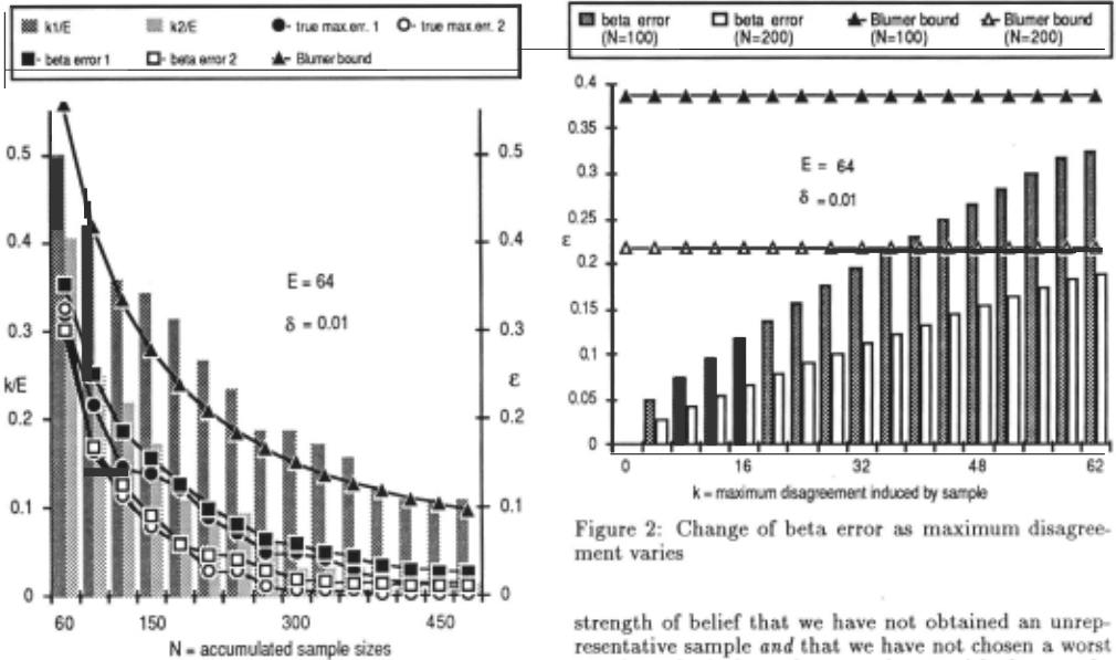
from E = 64 distinct classified examples. The Blumer bound given assumes the hypothesis space is complete. Notice how the beta error decreases with the maximum disagreement, i.e. when more example types are seen in the sample, consistent hypotheses will have lower error. This demonstrates just how important it is to make use of knowledge about a sample when evaluating PACness.

5 Average rather than worst case PACness

The use of the bound obtained in Lemma 1 or the Blumer bound, as with Haussler's notion of f-exhausting a hy­ pothesis space [Haussler, 1988], are really worst case analyses: they apply to every consistent hypothesis. If we choose a single consistent hypothesis arbitrarily, then we may choose a worst case, or we may choose a more ac­ curate hypothesis. To see what is wrong with this worst case analysis, suppose we have a carton of 200 apples, of which at most 3 are known to be bad. According to a worst case analysis, we cannot be confident of picking a good apple out of the carton because in the worst case we will get a bad apple. An average case analysis, like common sense, tells us that if we pick an applt out of the carton, we can be confident (98.5% in this case) it will be a good apple.

To introduce an average case analysis, we could, for instance, determine the confidence 1 - 8 that error is at most f for an arbitrarily chosen consistent hypoth­ esis, bearing in mind that some consistent hypotheses may have a worse error. This confidence represents our strength of belief that we have not obtained an unrep­ resentative sample and that we have not chosen a worst case hypothesis from those consistent with the sample. Both are chances we have no control over.

6 Considering preferences on hypotheses

As mentioned above, the classical interpretation and the result in Lemma 1 give confidence on error bounds for the worst case consistent hypothesis. In practice, of course, we do not build induction programs that try to find the worst conjecture consistent with the sample, nor do we arbitrarily choose one. Most induction practitioners spend their time trying to find a conjecture that they believe is in some sense the best. How should this be done?

Merely choosing just any consistent hypothesis may ignore vital information of a form not able to restrict the hypothesis space. Suppose, as Littlestone considers [Littlestone, 1988], we suspect there are abundant irrel­ evant or ,redundant attributes . It would be an obscure application where we know exactly how many attributes are irrelevant or redundant . Suppose, as Rivest consid­ ers [Rivest, 1987], we believe decision lists form a suit­ able hypothesis space. Do we use 5-DL (decision lists with conjunctions of size 5 at each decision) or maybe 10-DL? In fact, this is what we typically want the in­ duction system to tell us. Suppose we make a guess and consider a hypothesis space of r-DL. If we undershoot on r, we may end up finding no consistent hypothesis at all. If we overshoot, there may be many hypothesis left consistent with the limited sample we do have, and we have no assurance that an arbitrarily chosen one will have a suitable measure of PACness. Clearly, we should not choose such a hypothesis arbitrarily.

This issue has caused Mitchell to propose the need for "bias" in induction [Mitchell, 1980]. Bias is infor­ mation extraneous to the sample used when choosing a hypothesis. For instance, we might choose a hypothe­ ses that is "preferred" in some sense. In the situation above, if we believe irrelevant attributes abound, we might search for a consistent hypothesis that incorpo­ rates a smaller number of tests, for instance, a shorter decision list. An early paper by Gold [Gold, 1967] gave a result that supported Mitchell's proposal. Gold showed that there is no logic learning algorithm that uniformly requires a smaller number of examples to correctly iden­ tify a hypothesis than the "identification by enumera­ tion" algorithm. Since almost all reasonable logic learn­ ing algorithms can be classed in this broad category, we can conclude that some algorithms perform well on some types of problems, others perform well on other types of problems, but no algorithm performs uniformly better . As a consequence, the best we can do in logic induction is to hope that we choose an algorithm that performs well on the style of problem we are presented; and only information extraneous to the sample can help us in this choice.

The approach used by many applied logic induction systems is to use Occam's razor as a "preference order­ ing" on hypotheses. These systems search for "simpler" consistent hypotheses where the notion of simple is a syn­ tactic notion relative to the description language chosen for the application. For instance, Quinlan's ID3 [Quin­ lan, 1986] does this by searching for a more compact de­ cision tree consistent with the sample. As a result, the ID3 algorithm could not be expected to perform well, for instance, in learning some DNF formulae. These can have quite complex decision tree representations.

Notice that this use of a preference ordering must be relative to the application concerned because any syn­ tactic measure is a language dependent concept, and the language used is typically supplied by a domain expert. Caution also dictates that we only use an ordering that we have some prior justification for, otherwise we may as well arbitrarily pick a consistent hypothesis. Gold's result also assures us that this is the best methodology available when learning logic concepts. Finally, the clas­ sical and the two revised PACness notions are now in­ appropriate because they do not account for the use of preferences.

7 The Bayesian approach

The only induction theories that address the use of pref­ erence (or "bias") specifically are Bayesian statistics and its logarithmic counterpart, the minimum description length (MDL) method. These answer Mitchell's con­ cerns [Mitchell, 1980] in mathematical detail: how "bias" is required, how it can be implemented (as a measure of belief), and how it effects the logical induction process. The Bayesian approach is discussed here.

For each hypothesis HE 1i, we have Pr(H) an a pri­ ori measure of belief in it being "true" before the sample S is seen, and Pr(H I S) an a posterior measure of be­ lief after the sample has been seen. The prior measure may be uniform for all hypotheses in the space; in which case we are using a non-informative prior, and acknowl­ edging that we have no basis to prefer one hypothesis other another. When using Occam's razor as a prefer­ ence ordering on hypotheses, we are tying the prior to some measure of hypothesis size.

For each hypothesis H, prior and posterior are related as follows:

It is quite simple to show that this relation holds even when a sample is made without replacement, or when ex­ amples are obtained through the learner making queries. The relation shows that the prior preference ordering we choose before obtaining the sample is also appropriate, given a sample, for ordering those hypotheses consistent with the sample.

It is implicit in the current interpretation of the Valiant model and in the MDL model that we should choose just a single consistent hypothesis to make pre­ dictions with. To be more in the spirit of the Bayesian approach, we should instead choose several of the "bet­ ter" hypotheses and pool their predictions, as a means of "hedging our bets" . This is a consequence of the de­ cision theory component of the Bayesian approach. Ex­ periments show this hedging of bets may give only minor improvement in subsequent prediction accuracy, but c_an also lower the variance of prediction accuracy for classifi­ cation rules built from different samples (Buntine, forth­ coming).

The Bayesian approach also gives a method for deter­ mining confidence in error estimates, for example, PAC­ ness. This method does not appear to suffer the three broad problems claimed earlier about the Valiant model. For the classification rule C to be used, we first need the mean error f according to posterior belief, J1C (f), representing how much error we expect C to have, and the variance of this error, ub (f), representing our uncer­ tainty in the expected error. For the case of a random sample and the so called non-informative prior (a = t) these quantities are as follows:

where k( C, H) represents the disagreement between C and H which is the number of classifications out of all possibl~ distinct examples on which C and H disagree, and N and E have their usual meaning 2 . The mean error is calculated as the average disagreement divided by 2N +E. The mean and variance could be approximated stochastically by finding a small number of hypotheses consistent with the sample and then evaluating the two summations in the above equations on these hypotheses. PACness can then approximated from these quantities.

2 These equations follow using the method of proof for Lemma 1 and knowledge of the mean and variance of the beta distribution.

8 Conclusion

It has been argued that analysis of learning algorithms would better consider how to search for one or several preferred consistent hypotheses, and that prediction er­ ror can be approximately bounded using the sample de­ pendent quantities maximum disagreement and average disagreement. These quantities play the role of log l1il in the Blumer bound .

The following open problems illustrate the kinds of computational issues that need to be addressed to de­ velop the Bayesian approach given here in the manner of Valiant's [Valiant, 1985] broad learning framework .

1. How can maximum disagreement or some average measure of disagreement be efficiently estimated for samples from different concept classes?
2. The analysis in Sections 4 to 7 consider how to more accurately determine PACness given a sample, but not how large a sample is initially required. How is maximum disagreement or some average measure of disagreement expected to grow with the sample size, or what is Pr(k I N)?
3. What are suitable algorithms and what is the com­ putational complexity of searching for "preferred" consistent hypothesis for various concept classes and preference criteria? Both Haussler [Haussler, 1988, Section 5] and Rivest [Rivest , 1987, Section 5.3] have briefly considered this question using "simplicity".
4. Just how good is the stochastic approximation for determining PACness (outlined in Section 7) under a range of different priors and concept classes?

If current trends on applied machine learning are any guide, then even more interesting problems revolve around the learning of uncertain concepts.