Reasoning About Assumptions in Graphs of Models

1 Introduction

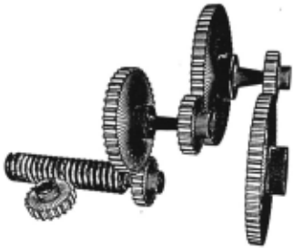
An important a.'>pect of real-world problem solving is the ability to represent, and reason with , large amounts of domain knowledge. For example, intelligent analysis of the transmission shown in figure 1 requires thorough knowledge of about three sophisticated textbooks (e .g. [Martin, 1982], [Arges and Palmer, 1963], [Boston Gear Co., 1960]) . Unfortunately, declaratively representing large amounts of knowledge leads to several problems; e.g. many knowledge-base operations, such as inference and checking consistency, are typically exponential in the size of the knowledge-base.

One approach to dealing with the complexity of large scientific and engineering domains is to make assump­ tions on the world. Making assumptions permits the decomposition of large domains into several smaller knowledge-bases called models ([Murthy and Addanki, 1987], [Falkenhainer and Forbus, 1988]). A model may be used in lieu of the larger domain knowledge-base if its assumptions lead to an acceptable approximation of the world.

The goal of the decomposition is to simplify problem­ solving by permitting analysis in the simplest model that is an acceptable approximation of the world. Ideally, the appropriate model should be identified before the start of analysis. However, in many cases, the inadequacy of a model becomes evident only through trial and error. Therefore, it is crucial that problem-solving paradigms based on models include mechanisms for automatically and efficiently selecting a better model when analysis in the current model is found to be in error.

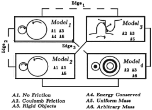
In our paradigm, called Graphs of Models, models are linked by directed edges . The edges specify how the assumptions of the source model change in going to the destination model. Figure 2 shows a part of a simplistic graph of models for the domain of transmissions. Our paradigm includes methods that automatically change models when the current model is inadequate. A brief example will help motivate our methods.

Let us start an analysis of our transmission (figure 1) using Modell of figure 2. Modell makes the assump­ tions that there are no frictions in the world, that all objects are rigid, that energy is conserved, and that all masses are uniformly distributed. As Modell is not an acceptable approximation of the world, it predicts a rotational acceleration value that is higher than the experimentally observed value. This error, or conflict, invokes a reasoning process in which Modell first anal­ yses the conflict to find that the error is due to forces that have not been accounted for. Next, Modell uses domain knowledge about its assumptions to find that an assumption change, or transition, from no frictions to coulomb frictions introduces new forces that cause ac­ celerations to decrease. Finally, Modell finds the edge that best matches this assumption change, Edge 1, and transfers control to the model at the end of this edge.

This process requires four abilities. The ability to de­ tect conflicts, the ability to determine how parameters must change in order to eliminate conflicts, the ability to represent how assumption transitions affect parameters in the world, and the ability to use this knowledge in selecting the next model.

We introduce the notions of delta-vectors to cap­ ture the qualitative nature of parametric changes that will eliminate conflicts 1 , and parameter-change rules to capture domain-level knowledge about how assumption transitions affect values of parameters. A simple in­ ference mechanism uses delta-vectors and parameter­ change rules to decide which assumptions to change. In­ tuitively, delta-vectors may be seen as goals that have to be achieved, assumption transitions as the actions that will satisfy these goals, and parameter-change rules as the post-conditions of these actions. The mechanisms are qualitative in that they are based on the ( + - 0) cal­ culus of [deKleer and Brown, 1984] and [Forbus, 1984]. They have been used in four implementations of Graphs of Models in the domains of Mechanics, Thermodynam­ ics, Fluids, and Geometric Structure.

Section 2 presents more details about Graphs of Mod­ els. Section 3 describes conflicts and how we detect them. Section 4 describes delta-vectors and how they are computed. Section 5 describes how parameter-change rules represent knowledge about assumptions and Sec­ tion 6 describes the inference methods used for changing assumptions. We end the paper with a few of the many questions that we still have to address and the relation­ ship of our work to others.

2 Graphs of Models

Making assumptions on the world permits organized re­ formulations of domain knowledge that are much like models in the scientific or engineering sense of the term. A model, in our paradigm, may make fifteen to twenty assumptions and consists of two parts. The first per­ forms analysis within the model and the second deals with changing assumptions. A brief description of the first part follows. The second part is the focus of this paper.

1 For this paper we will assume that all conflicts arise from incorrect values or expressions for physical parameters.

(defrule netl (rigid-object :=obj :=t) (net-torque :=obj = r ::axis :=t) (net-angular-acceleration ::object ::a :=axis :=t) (moment-of-inertia ::obj =I ::axis :=t) => (net-acceleration-equation :=obj :=eqn :=vars :=t) (compute ::eqn "::a= ::r/::1") (compute ::vars "[::a]"))

The analysis part of a model contains a knowledge­ base of rules in a first-order-like language. The rules are exactly the rules of physics found in textbooks. The rule in figure 3 describes the simple a = ] law of rotational dynamics; a is rotational acceleration, r is net-torque and I is rotational inertia. The language is based on a sorted calculus and the predicates are strongly typed . The sorts constitute the ontology of the world and are organized into a hierarchy. The last parameter of e~ery predicate is a temporal variable that refers to a time point or interval over which the proposition is valid. The temporal entities are supported by a powerful single time line reasoner described in [Penberthy, 1988]. The language supports expressions that may be executed by LISP or passed to MACSYMA [Martin and Fateman, 197~] for further evaluation; values of parameters are numen­ cal values or symbolic expressions. Analysis consists of natural deduction that is tightly controlled by model­ specific heuristics.

The principal advantage of a model is its specificity. A model addresses a relatively narrow scope of phenom­ ena. Typically, models are much smaller than the entire domain knowledge. It is relatively easy to represent the knowledge that is valid within a model. Further, the specificity helps define very efficient model-specific anal­ ysis methods. Some apparent contradictions to these claims turn out to be deceptive. For example, Maxwell's equations and N a vier-Stokes equations are very compact and appear to define all the domain knowledge for elec­ trodynamics and fluid flow respectively. However, it is very hard to use either sets of equations, in practi­ cal analysis, without making several assumptions on the world.

Domain knowledge is represented as a Graph of Mod­ els. The typical Graph may have tens of models. The Graph of Models of a domain is complete; all models have edges to all other models. A typical edge has around five assumption transitions. For each model, the edges leading to other models are grouped into prior­ ity classes. The priorities al~m~ a "distance" . meas~re in a complete graph by spec1fymg the order m wh1ch the edges are searched when changing models; "near" edges are searched before "far" edges. The Graph of Models of a domain is sparse; the graph does not con­ tain models for every combination of assumptions in the domain. The models that are contained in a Graph of Models are called "materialized models" , other combina­ tions of assumptions are called "non-materialized mod­ els" . It is obviously better to dynamically reconfigure models based on the exact set of assumptions required. Unfortunately, early work on reformulation of theories shows that this is not easy to do ([Subramanian and Genesereth, 1987], [Lowry, 1987]).

3 Conflicts

In our current approach conflicts can occur in three ways: Empirically, Internallly, and through Inter-domain in­ teraction . An Empirical conflict is a mismatch between the value of a parameter predicted by a model and the value measured in the world. Empirical conflicts arise in experimentally verifying a model's predictions; e.g., the conflict, described earlier, in the acceleration of the transmission. Internal conflicts occur when a value de­ rived within a model violates one of the model's as­ sumptions. For example, Model 1 makes the Conser­ vative Systems and the Rigid Bodies assumptions. If the Rigid Bodies assumption is inappropriate, the predicted values for energy will violate the Conserva­ tive Systems assumption. Inter-Domain Conflicts oc­ cur when multiple domains interact in analysing a device and two or more domains disagree over the value of a common parameter [Addanki et al. , 1989].

Parameters can be numerical values or constraints. Hence conflicts take one of the following forms : Numerical-Numerical, where both values are numeri­ cal; Numerical-Constraint, where one value is numeri­ cal and doesn't satisfy the constraint; and Constraint­ Constraint, where both values are constraints that are unequal.

Detecting empirical conflicts is a straightforward pro­ cess . At the end of the analysis session the system asks the user to verify its predictions. The user gives the system his/her set of values for the parameters and the system compares its predictions against the user's mea­ surements. Detecting internal conflicts is a little more difficult and requires knowledge about the assumptions in the form of consistency rules (section 5.1) . The detec­ tion of inter-domain conflicts is described in [Addanki et al. , 1989].

4 Delta-Vectors

Delta-vectors represent the qualitative changes, to pa­ rameters values, that will eliminate a conflict . A delta­ vector is an ordered pair ; the first element is the name of the parameter in conflict and the second element is a qualitative vector representing the required change. This follows our representation of vectors as a magnitude and a direction unit vector. In our example the delta-vector for the acceleration of the transmission is (a, (- {000))) where the minus sign (-) signifies that the magnitude of the acceleration is to be reduced and the {000) signifies the direction of the acceleration is correct . When more than one parameter is found to be in conflict, the delta-vectors are stored as a list called the delta-list.

4.1 Computing Delta-Vectors

Delta-vectors are first computed for the parameters ac­ tually in conflict. This delta-list is called the base-delta­ list. The same mechanisms are used for computing delta­ vectors for empirical, internal, and inter-domain con­ flicts.

Computing delta-vectors in a Numerical-Numerical conflict consists of computing the difference of the em­ pirical vector and the predicted vector and taking the signs of the result . In our example if Modell predicts a= {10.34 {000)) and a is measured to be {8.27 {000)), the delta-vector is (a, (- {000))).

There are two types of Numerical-Constraint conflicts . In one the constraint is Causal; i.e. it is an equation or inequality that is established by a model to compute a parameter in terms of others. It is usually derived from a physical law. In our example, Model 1 sets up the equa­ tion a = :!. to compute a. The other constraint is Im­ plicit, a pfiysical principle that must be satisfied by the parameters of the model. Examples are the conservation of energy and momentum in Mechanics and pv = nRT in Thermodynamics. Implicit conflicts are usually internal conflicts. Note that the difference between causal and implicit is in how a constraint is used by a model, and is not inherent in the constraint.

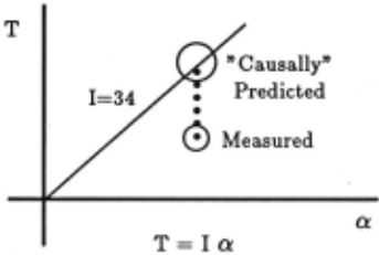
If a predicted causal constraint fails to match a mea­ sured value, the model has already used the constraint to compute its value for the parameter while detecting the conflict. This value is used to set up a vector-vector con­ flict with the measured value (see figure 4). For example, Modell predicts a = f . Empirically a is {0.43 {000)) for T = {27.0 (000)), and I = 34.0. In detecting the conflict Model1 has already computed a'= {0.79 {000)) for T = {27.0 {000)) and I = 34.0. Modell treats a' as the predicted value and a as the measured value in a vector-vector conflict. The resulting delta-vector is (a, ( -{000))) . Note that delta-vectors say nothing about how a constraint is to be changed; they only indicate how the value of a parameter is to be changed.

The method fails when the measured value is outside the domain of the constraint; e.g. when the constraint is y = }9- x 2 , and the value measured is {5, 5) . In

.

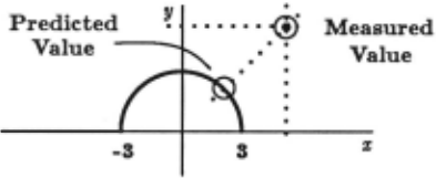
such situations the model exploits the fact that delta­ vectors can only specify the quadrant 2 into which, or the axis along which, the change should be made; where the quadrants are with respect to the measured value. Delta­ vectors are computed by setting up artificial vector­ vector conflicts between the measured value and artifi­ cial predicted values. The artificial predicted values are generated by finding intersections of the lines that pass through the measured point, parallel to the axes, with the predicted constraint. Each point of intersection is an artificial value. Intersections beyond a region pre-defined by the user are ignored. If no intersections are found the constraint lies entirely within a quadrant and a single ar­ tificial point is generated by assigning values arbitrarily to the parameters of the constraint. In our example, the lines y = 5 and x = 5 do not intersect the constraint. Hence an arbitrary value, say {0, 3), on the constraint is selected and is set up as a vector-vector conflict with {5, 5). This results in a delta-vector of (y, ( + )}.

Detecting constraint-constraint interactions, if the constraints are linear, is polynomial; if the constraints are algebraic the problem is exponentially space com­ plete; if the constraints include transcendentals the prob­ lem is uncomputable. Currently our models handle the very limited classes of constraint-constraint conflicts in which one constraint is strictly greater than the other. However, many constraints fall into a few specific classes for which special purpose routines can check for differ­ ences in order, coefficients, phase, etc. For example, special purpose heuristics can resolve constraints on cur­ rents propagated through a circuit [Stallman and Suss­ man, 1977] . Similarly, many constraints on a single tran­ scendental variable, e. g. x sin( 8) ~ k, can be handled with a quadrant calculus that assigns signs to the tran­ scendental functions in each quadrant; e.g., sin(O) will be represented as ( + + --) for the four quadrants. We are in the process of developing such algorithms.

In computing delta-vectors for implicit numerical­ constraint conflicts the model directly generates artifi­ cial predicted values to compute the delta-vectors. The first stage is ommitted due to the the lack of a causal relationship.

The preceding discussion assumed that the model gen­ erated only one constraint that consisted of a simply­ connected portion of space. The methods generalize easily to multiple constraints if a simply-connected fea­ sible solution space exists. Disconnected pieces, e.g. xy = 1, are handled by the artificial vector-vector conflict method with the points of intersection being com­ puted by a stepwise sweep of a line passing through the measured value. The resolution of the angular step is de­ creased iteratively until points of intersection are found .

2 0ctants for 3-space.

The methods generalize to more dimensions. The dis­ cussion also assumed that the model predicted a con­ straint that was not satisfied by a measured value. The same methods apply if the model predicts a value that does not satisfy a constraint measured in the world.

4.2 Extending the Delta-List

The model also has to account for errors in intermedi­ ate parameters used in deriving the actual parameter in conflict. For example, an error in r, an intermedi­ ate parameter, will cause an erroneous value for a. The base-delta-list is extended to include these parameters and the final list is called the extended-delta-list.

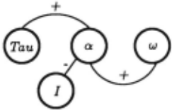
Our models maintain a detailed proof graph of the analysis. Backtracking through this graph finds all the parameters that affect the parameters in conflict. Each model also explicitly represents known parameter depen­ dencies; e.g., force affects acceleration, that in turn af­ fects velocity, etc. These dependencies are represented as influences, [Forbus, 1984], in semantic nets called In­ fluence Nets (1-Nets). A sample 1-Net containing the in­ fluences between torque, acceleration, and other param­ eters in solid dynamics is seen in figure 6. The required change (or delta vector) of the parameter in conflict is propagated through the 1-net to determine the corre­ sponding changes in intermediate parameters. 1-nets help finesse the problem of back-propagating a change through complex equations.

In our example, the extended-delta-list Js: {(a,(-{000))}, (r,{-(000))}, (!,+}} whereawasthe only parameter in the base-delta-list .

5 Assumption Knowledge

Assumptions affect the behaviors we expect to see in the world. For example, the coulomb frictions assumption requires that if two objects are in contact at a surface a force prevents relative sliding of the objects, that sys­ tems are dissipative, that heat be generated, and it also specifies the orders of magnitude of these effects. We rep­ resent two kinds of knowledge about assumptions, Con­ sistency Rules and Parameter-Change rules.

5.1 Consistency Rules

Often, for ari assumption to be valid, the parameters must satisfy given consistency constraints. For example, in Modell, the conservative systems assumption requires that the energy within the system being ana­ lyzed remain constant. The ideal gases assumption specifies a fixed constraint between the pressure, the volume, the mass, and the temperature of gases in the world. The laminar flow assumption in fluid dynamics requires that the Reynolds number of the flow remain below 2300. These constraints are represented as con­ sistency rules that are checked periodically throughout analysis. An inconsistency is an internal conflict (dis­ cussed in section 3) and invokes the model changing ap­ paratus.

(Defrule add-friction-! (solid-object :=o1 :=i1) (solid-object :=o2 :=i1) (surface-of-contact :=o1 :=o2 :=surf1 ::i1) (net-force :=o1 :=nf1 :::i1) (force-component :::nf 1 :=surf! ::: /p :::il) => (parameter-change ::: fp = dvector1 :::i1) (compute :=dvector1 £'(+)))

5.2 Parameter-Change Rules

Parameter-change rules represent the qualitative effect of assumption transitions on parameter values. Transi­ tions typically have four to six parameter-change rules. The rule in figure 7 is taken from the no-frictions to coulomb-frictions transition. It asserts that if two ob­ jects are in contact at a surface, there is an increase in the component of the net-force along the surface of contact. The antecedents of the rule describe the con­ figuration of the objects and define /p to be the compo­ nent of net-force parallel to the surface of contact. The parameter- change predicate in the consequent says that /p changes by amount dvector1 . The compute predi­ cate tells how to compute the amount of the change; the amount of the change is ( +), a qualitative increase in /p under the transition. When applied to gear train trans­ missions, this rule represents an overall decrease in the effective force used to transmit torques. A simpler rule, useful in our example, states that if two gears are meshed there is a decrease in the magnitude of the net-torque on both gears.

The antecedents of rules describe situations in which parameters are affected by the assumption transition. The language of the antecedents is exactly the same as the domain language. The situation is quite specific in describing the conditions under which the parameter­ change may occur; this permits problem-specific selec­ tions of assumption transitions. In our example, the an­ tecedents required objects to be in contact. Hence, the transition can be rejected when the object of interest is not in contact with another object but a decrease in its net-force is still required.

The consequents describe the parameters that change and how they change. The language of the consequents introduces the parameter-change predicate. The pa­ rameter change may be simple, as in a qualitative (-) or ( +), or complex, as in any LISP or MACSYMA state­ ment in the compute predicate. The consequent may introduce a parameter that is not part of the vocabulary of the current model. For example, a simple no fric­ tions model of dynamics may not include heat. Such parameter-change rules are used for matching against assertions from other domains or from the user. In our experience, the situations in the antecedents can get complex but the computations in the consequent stay as simple as the inner product of vectors.

6 Selecting a Better Model

Recall that the edges away from a model are grouped into priority-classes. Selecting a better model consists of stepping through these classes, searching each for an acceptable edge. For each step, the delta-vectors specify the desired changes in parameter values, the assump­ tion transitions are actions that realize these goals, and the parameter-change rules specify how the transitions affect parameter values. The final step, invoked if no acceptable edge exists, determines the combination of assumption transitions that best satisfies the delta-list; this helps automate extending the Graph. An overview of the algorithm that selects a model from a given prior­ ity class is described in figure 8. The reader may find it useful to refer to figure 8 for definitions of terms intro­ duced in this section.

1. Calculate the Candidate Transition Set (CTS) through goal-directed search on Parameter-Change rules. The CTS contains a set of assumption transi­ tions, each of which satisfies at least 1 delta-vector .
2. Create a Transition Satisfaction List (TSL) for each assumption transition in the CTS. The TSL of a transition specifies how well the transition satisfies each of the delta-vectors.
3. Create an Edge Satisfaction List (ESL) for each edge by qualitiative addition of all TSL's within an edge. An ESL of an edge indicates how well the edge sat­ isfies each of the delta vectors.
4. Create a Candidate Model Set (CMS) by choosing those edges with satisfactory ESLs. The CMS is a set of possible alternative models.
5. Choose a model from the CMS whose assumptions are consistent with the problem statement.

Figure 8: A summary of our model selection algorithm

The model starts with the highest priority class of edges. The first step is to find those assumption tran­ sitions that satisfy at least one element of the delta­ list. Each edge consists of a: set of assumption transi­ tions. Each transition has a set of associated parameter­ change rules. The model collects all these parameter­ change rules into a temporary knowledge-base. The model then matches every delta-vector in the delta-list against the rules in this knowledge base. When the consequent of a rule specifies a parameter change that matches a delta-vector, the model attempts to match the situation in the antecedent of the rule against the current description of the device. If the antecedents match immediately, the assumption transition associ­ ated with this rule is placed in the Candidate-Transition­ Set (CTS). 3 At the end of this backward-chaining the CTS contains all the assumption transitions that sat­ isfy at least one delta-vector. In our example, Modell has three edges leading away from it and they are all in the same priority class. Two transitions match; no frictions to coulomb frictions matches (r, (-(000))} and uniform-mass-distribution to arbitrary-mass­ distribution partly matches (I,+}.

The model maintains a transition-satisfaction-list (TSL) for each assumption transition in the CTS. The TSL of a transition specifies how well the transition sat­ isfies each of the delta-vectors in the delta-list. A TSL has as many elements as the delta-list has delta-vectors. Each element is (+), (-), (0), or (C). A (+) in the nth place indicates that the transition satisfies the nth delta-vector, a (-)that it violates it, a (0) that it doesn't affect it, and a (C) that it does change the parameter but the direction of change is unknown. At this stage the elements of the TSLs are either ( + )s, ( C)s or (O)s because the backward-chaining finds all the positive ef­ fects of the transitions. The TSLs are also divided into two parts, one for the base and the other for the ex­ tended delta-lists. Recall that the base-delta-list con­ tains a and the extended-delta-list contains rand/. The TSL for the frictions transition is {(a\0), (r\+, I\0)} and the TSL for the mass-distributions transition is {(a\0), (r\0, 1\C)} .

The model then finds all the negative effects of the transitions in the CTS by forward-chaining through their parameter-change rules . This is also a one step pro­ cess . These violations are stored as (-)s in the TSL of the transitions. Our simple example does not include any violations. The next step .is to check if the I-Nets show that any non-(0) parameter in a TSL influences a (0) parameter in the same TSL. Such an influence may cause the (0) parameter to be satisfied or violated by the transition. In our example, the I-Net in figure 3 shows that T, ( +) in the frictions TSL, affects a, (0) in the same TSL, positively; hence the transition also satisfies the delta-vector for a. The value for a in the frictions TSL is thus changed to ( +) and the TSL now reads {(a\+), (r\+, l\0)}. Similarly, since the I-Net shows that I affects a inversely, the TSL for the mass­ distributions TSL now reads {(a\C), (r\0, 1\C)}. At this point the TSL of each transition in the CTS provides a composite picture of how well the transition satisfies the delta-list .

The next step is to compute a similar composite picture of how well each edge satisfies the delta-list. The edge-satisfaction-list (ESL) of each edge in the highest priority class is computed by vector addition of the TSLs for each of the transitions in the edge; the rules of ad­ dition are the standard rules of the ( +, -, 0) calculus with (0) being the ambiguous condition (see [Forbus, 1984], [deKleer and Brown, 1984]). A (C) added to any­ thing gives a (C). Like the TSLs the ESLs have two parts, one for the base- and the other for the extended­ delta-lists The ESLs for the three different edges out of Modell are Edge1 : {(a\+), (r\+, 1\C)}, Edge2: {(a\0), (r\0, I\0)}, and Edge3 : {(a\C), (r\+, 1\C)} (see figure 1).

3 We require that the antecedents match immediately, with no further backwa,rd-chaining. If the powerful problem solv­ ing mechanism in the model did not discover the situation in the antecedent, it is unfair that the assumption reasoner be asked to do so. It is clear that there will be cases where the limitation will restrict the power of the system.

In evaluating the ESLs to select the next model, recall that the actual conflict involved only those parameters in the base-delta-list. If the ESL for the base-delta-list of any edge is perfect, i.e. all ( + )s, the model at the end of that edge is placed in the Candidate Model Set ( CMS) for consistency checking. If the CMS is non-empty, the consistency rules of each assumption in each model in the CMS are checked against known parameter values. This eliminates moving to models which may satisfy the delta-list but are inconsistent with the system being an­ alyzed. Finally, one of the remaining models in the CMS is selected arbitrarily. We do not have to look at edges in the other priority groups because we cannot do better than a perfect ESL that meets all the consistency re­ quirements . If the CMS is empty, the TSLs are used in repeating the process for edge groups of lower priorities. In our example, the ESL for Edge 1 satisfies it. Model3, at the end of Edge1 is placed in the CMS. The current parameters satisfy the consistency rules of Model3 and it is chosen as the next model.

If no existing edge provides a perfect match, the model picks the next best match from all its edges. ESLs are evaluated numerically:(+)= +1, (-) = -1, (C)= 0.5, and a (0) = 0. Adding the elements of an ESL results in a numerical "goodness" value for the edge. 4 The models at the end of the edges with the highest goodness values are placed in the CMS. The CMS is filtered for consistency, and the next model is selected from the filtered CMS.

Before control is transferred to the selected model the model has the option of checking all combinations of as­ sumptions to see if a better match can be found. Recall that the Graph of Models is sparse and hence does not include materialized models for every combination of as­ sumptions. Checking to see if a non-materialized model results in a better match is useful for automating the process of extending a Graph of Models. Unfortunately the process is NP-complete; it is reducible to test-set generation.

7 Conclusions and Future Work

Four implementations, albeit limited to domains con­ taining four to eight models, in Geometric Structure, Thermodynamics, Mechanics, and Fluids, lead us to be­ lieve that the Graphs of Models paradigm is a powerful approach to representing complex, scientific and engineering domains. Much of the power of the paradigm comes from its methods for automatically changing mod­ els. The qualitative mechanisms of delta-vectors and parameter-change rules provide powerful and efficient model changing behaviors .

4 This is a very simplistic measure of "goodness" and we are testing its limitations.

However, the mechanisms are limited in many ways. One important limitation has to do with the paucity of information in parameter-change rules. For exam­ ple, humans typically use much Order of Magnitude in­ formation while evaluating the effects of changing as­ sumptions. In our example, a human expert would com­ pare the order of magnitude of the change due to fric­ tions with the difference between the predicted value and the measured value of the acceleration. The diffi­ culty with using existing approaches to order of mag­ nitude reasoning, e.g. [Raiman, 1986], [Mavrovouniotis and Stephanopolous, 1987], or [Murthy, 1988], is in set­ ting the threshold for the comparisons. These thresholds are problem-dependent and have to be set dynamically, an open problem at this time.

The mechanisms are also limited by the simplistic na­ ture of building and comparing ESLs. Domains typi­ cally contain much more information about the utility of models in a given situation . This information may be in terms of tests that can be carried out to check the validity of a change, empirical likelihoods of assump­ tion transitions, knowledge about parameter behaviors as computed in the current model, and so on. The cur­ rent mechanisms make no use of any of this information. A large part of our future work will focus on building rep­ resentation and inference mechanisms for handling these types of knowledge.

The use of assumptions to simplify problem-solving is not new. It is an inherent part of science and en­ gineering. In the AI literature, [deKleer and Brown, 1984] emphasize the importance of making modelling assumptions explicit and acknowledge that the prob­ lem of changing these assumptions is an important one. [Murthy and Addanki, 1987] suggest the Graph of Mod­ els paradigm but present few details on its internal work­ ings. [Falkenhainer and Forbus, 1988] re-emphasize the importance of using assumptions to decompose complex domains into simpler models but do not indicate how control is transferred from one model to another. The­ oretical approaches such as [Lowry, 1987] and [Subra­ manian and Genesereth, 1987] have attempted to dy­ namically reconfigure theories based on the exact set of assumptions required, but the results have been of lim­ ited applicability to complex knowledge bases. For ex­ ample, [Subramanian and Genesereth, 1987] require that the entire problem be solved before deciding what parts of the knowledge base are irrelevant. Finally, in spite of its limitations we believe that a rigorous (though empir­ ical) approach such as the Graph of Models paradigm provides a powerful technique for representing physical domains.