Stochastic Analysis of Qualitative Dynamics

1 Introduction

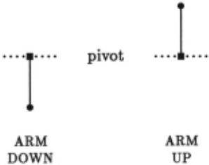
Qualitative reasoning seeks to predict the global behav­ ior of a complex dynamic system by partitioning its state space into a manageable number of qualitative states and characterizing its behavior by the sequences of qualita­ tive states that it can go through. This methodology is too weak to describe the limiting behavior of dynamic systems. For example, a damped pendulum eventually must approach equilibrium either directly below or di­ rectly above its pivot (Figure 1) . The first possibility is almost certain, whereas the second almost never occurs. Qualitative simulation discovers both equilibria, but can neither determine their relative likelihoods nor rule out Elisha P. Sacks Department of Computer Science Princeton University Princeton, New Jersey 08544, USA

· Authors listed alphabetically. Jon Doyle is supported by the National Library of Medicine under National lnstitu tes of Health Grant ROl LM04493.

the possibility that the pendulum will spin forever. Yet qualitative considerations suffice for both conclusions, independent of the numeric details of the system.

Limiting behaviors are global characteristics of a sys­ tem. To understand them, we must look beyond indi­ vidual transitions to sequences of transitions. We must assign each sequence a likelihood, ranging from impossi­ ble to definite. In this paper, we describe one approach to this problem. We estimate the likelihoods of a sys­ tem's asymptotic behaviors by viewing its dynamics as a Markov chain over its transition graph. This corre­ sponds to adding probabilities to each of the transitions. The transition probabilities follow directly from theoret­ ical considerations in simple cases such as the pendulum example. In the remaining cases, one must derive them empirically from numeric simulations, experiments, or subjective estimates.

The standard theory of Markov chains provides exten­ sive information about asymptotic behavior, smoothly blending qualitative and quantitative information into a unifying framework that provides the best possible con­ clusions given the evidence. It derives some sorts of es­ sentially qualitative conclusions that qualitative simula­ tion does not, including a partition into persistent and transient states and a partition of the persistent states into the probable and the improbable. Many of these conclusions follow solely from qualitative considerations. The remainder, though numerically derived, are insen­ sitive to perturbations in the probabilities. The theory also provides quantitative refinements of these qualita­ tive conclusions, including the mean and variance of set­ tling times. Unlike the qualitative conclusions , the quantitative results are in some cases sensitive to variations in the input probabilities. The algorithms are straight­ forward, involving only a topological sort of the transi­ tion graph and a few matrix operations on the transition probabilities, and require time at most cubic in the num­ ber of qualitative states. The analysis goes through for symbolic probability estimates, although at the price of exponential-time worst-case performance.

2 Qualitative dynamics in phase space

The first step in our analysis of a system is to derive its states and transitions from the phase space of the system. The phase space for a system of first-order dif­ ferential equations

is the Cartesian product of the x; 's domains. One can convert higher-order equations to first-order ones by in­ troducing new variables as synonyms for higher deriva­ tives. Points in phase space represent states of the sys­ tem. Curves on which equation (1) is satisfied, called trajectories, represent solutions. A phase diagram for a system depicts its phase space and trajectories graphi­ cally. The topological and geometric properties of trajec­ tories characterize the qualitative behavior of solutions. For instance, a point trajectory, called a fixed point, in­ dicates an equilibrium solution, whereas a closed curve indicates a periodic solution. A fixed point is stable if ev­ ery nearby trajectory approaches it asymptotically and unstable otherwise. More generally, the stable manifold of a fixed point is the set of trajectories that approach it asymptotically. (See Hirsch and Smale [Hirsch and Smale, 1974].)

For example, the standard model for a damped pen­ dulum is

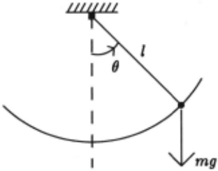
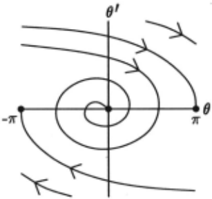
with (} the angle between the arm and the vertical, I the length of the (weightless rigid) arm, m the mass of the bob, g the gravitational constant, and J1. the damping coefficient, as shown in Figure 2. Figure 3 shows the pendulum's phase diagram. The symmetry and 27r pe­ riodicity of the pendulum equation make it natural to employ the cylindrical phase space obtained by identify­ ing the lines (} = -1r and (} = 1r . Two trajectories spiral toward the unstable fixed point at ( 1r, 0); the rest spiral toward the stable fixed point at (0, 0) .

A complete qualitative description of a system con­ sists of a partition of its phase space into sets of qualita­ tively equivalent trajectories. The equivalence criterion depends on the problem task. Mathematicians generally focus on topological equivalence, whereas coarser rela­ tions are more useful in engineering applications. We follow standard AI practice and equate all trajectories that go through a specific sequence of regions in phase space. Our qualitative dynamics consists of a partition of phase space into regions along with a graph of possible transitions between regions.

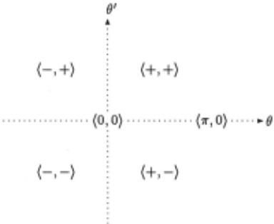
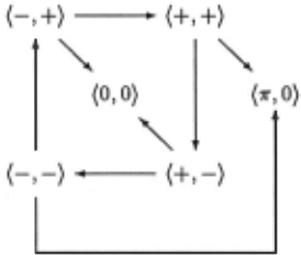
Sacks [Sacks, 1988c] shows how to translate traditional qualitative reasoning into our qualitative dynamics with­ out loss of information or increase in complexity. Quali­ tative states correspond to rectangular regions in phase space, and qualitative simulation amounts to finding the possible transitions between regions. A transition oc­ curs from region A to region B if the derivative of the system on the boundary between the regions points into B . A transition occurs from a region to a neighbor­ ing fixed point unless all the eigenvalues of the fixed point have positive real part, as explained in the next section. For example, automatic analysis of the damped pendulum equation results in six qualitative states corre­ sponding to four rectangles ( (±, ±}) and two fixed points ((0,0},(7r,O}), as shown in Figure 4. Figure 5 shows the transition graph over these qualitative states.

The probabilistic conclusions about the pendulum's asymptotic behavior follow from purely dimensional ar­ guments, which in turn may be determined by inspec­ tion of the eigenvalues of the fixed points. By the sta­ ble manifold theorem [Guckenheimer and Holmes, 1986, p. 13], the dimension of the basin of a fixed point equals the number of its eigenvalues that have negative real parts. 1 The real parts of the eigenvalues are both neg­ ative at (0, 0) and of opposite signs at ( 1r, 0). Hence, the basin of ( 1r, 0) has zero measure because it is a one­ dimensional submanifold of the two-dimensional phase space, whereas the basin of (0, 0) has positive measure. A similar argument shows the unstable equilibria of any system to be unlikely. But this approach is insufficient to yield all conclusions of interest in general, since systems may have multiple stable equilibria and other states with positive asymptotic probabilities.

1 This theorem applies to hyperbolic fixed points. The number of positive real parts at a.n arbitrary fixed point suf­ fices for our analysis.

3 Transforming flows into Markov chains

We estimate the likelihoods of a system's asymptotic be­ haviors by constructing a Markov process whose states are regions in phase space. The dynamic system it­ self is an uncountable Markov process whose states are the points of phase space, 2 but direct analysis or use of this Markov process is impractical. Instead, we lump the point-states into a manageable number of re­ gions in phase space, each of which represents a distinct qualitative state of the system. Sacks [Sacks, 1988a, Sacks, 19881:>, Sacks, 1988d] presents a system that auto­ matically identifies such regions and the possible transi­ tions between them for second-order systems of ordinary differential equations. Most of the ideas extend directly to larger systems. One can also work with the rectangu­ lar regions that qualitative simulation implicitly defines.

The second step in constructing the Markov process is to associate probabilities with each of the possible tran­ sitions between regions. These probabilities reflect the likelihood of the system's state moving from one state­ space region to another in unit time. We may obtain the probabilities directly from dimensional considerations in simple cases such as the pendulum example. Ordinar­ ily, though, they will come from numeric simulations or physical experiments that sample representative points in each qualitative region and count how many go to each region. In this procedure, stable equilibrium points must be represented by regions large enough to exhibit positive entry probabilities. Every stable attractor is surrounded by such a region, and one can be found by sampling with larger and larger small areas around the attractor. One can also obtain subjective estimates from domain experts. The qualitative analysis is insensitive to errors in these probabilities.

2 In fact, this Markov process is deterministic: all state transition probabilities are zero or one.

The transition probabilities represent the imprecision in the qualitative model of the dynamic system. If we were able to choose as regions the actual at tractors of the system, there would be no imprecision and the transition rules would be perfectly deterministic. The great diffi­ culty of determining the optimal set of regions for anal­ ysis helps motivate the stochastic approach to analyzing behaviors. Additional factors that transition probabili­ ties can model include (1) uncertainty about initial con­ ditions which induces a distribution of possible trajecto­ ries, (2) uncertainty about the parameters of the model equations, and (3) uncertainties (or noise sources) explic­ itly occurring in the system's equations, as in stochastic differential equations.

Our analysis treats the Markov process constructed from a dynamic system as a Markov chain. That is, we assume that the transition probabilities remain constant over time and that they depend only on the qualitative state of origin, independent of past history. The first as­ sumption holds for autonomous equations that are free of their independent variable. One can reduce any gen­ eral system to an autonomous one by treating the inde­ pendent variable, t, as a state variable governed by the equation t' = 1.

The second assumption holds to the extent that the fu­ ture trajectory of the system is insensitive to its distant past . The most questionable case is that of conserva­ tive systems in which the volume of each region in phase space is preserved for all time by the flow, causing small differences between trajectories to retain their signifi­ cance forever. Conservative systems pose problems for qualitative reasoning generally, not just for the stochas­ tic analysis, as the regions of interest must be chosen carefully. Fortunately, most realistic systems are dissi­ pative, hence volume shrinking, causing differences be­ tween trajectories to shrink exponentially.

Time-dependent transition probabilities imply that the current partition of phase space is too coarse: dif­ ferences within a prior region express themselves in the current region because the distances between points in the prior region are too great to damp out in one time step. One approach, following Sacks [Sacks, 1988a, Sacks, 1988b], involves iterative improvement of the model (though unlike that work, we have not automated this refinement process) . If one observes time-dependent behavior in constructing the transition probabilities, one subdivides or otherwise refines the set of regions and starts over. In principle, the process ends when the chain assumption appears correct for all regions, but in prac­ tice the choice of when to accept a model as satisfactory involves a tradeoff of model complexity against model accuracy. The aptness of the chain assumption can also be tested against empirical observations or long term nu­ meric simulations.

4 Analysis of Markov chains

In this section, we summarize the theory of Markov chains. The details appear in our longer paper [Doyle and Sacks, 1989] and in Roberts [Roberts, 1976]. Let S = { s1, ... , Sn} be the set of states of the qualitative dynamics, that is, the set of nodes of the dynamic di­ graph. Each of these will also be a state of the Markov chain. We describe the entire chain by specifying, for each nonexclusive choice of states s; and Sj, the transi­ tion probability Pii that if the system is in state s; at one instant, it will be in state Sj after one time unit has passed. We write P = {Pii} to mean the n x n transition matrix of all transition probabilities. P is also called a stochastic matrix, which means that all entries are non­ negative and that each row sums to 1. Each row of P is called a probability vector. The transition digraph of a stochastic matrix is the graph over the states with a directed arc from s; to Sj iff Pii f= 0.

The probability that the chain is in state si at time t given that it starts in state s; at time 0 is written p~J> and called a higher-order transition probabil­ ity. This probability is the i, j entry of pt, the t'th power of P. If we start the Markov chain at random, where the probabilities of starting in each state are given by an initial probability vector p(o) = (Plo), ... , p~ 0 )), then the probabilities of being in particular states at time t, p(t) = (Plt), .. . , p~t)), are given by the equation p(t) = p(O) pt.

A set C of states is closed if Pii = 0 for all s; E C and Sj rf. C, that is, if once in C the chain can never leave C . A closed set C is ergodic if no proper subset is closed. A state is ergodic if it is in some ergodic set, and is transient otherwise. A state that forms an ergodic set by itself is called an absorbing state. Chains whose states form a single ergodic set are called ergodic chains, and chains in which each ergodic set is a singleton are called absorbing chains.

The mathematical analysis of the asymptotic behavior of a Markov chain is divided into two parts: the behavior before entering an ergodic set, and the behavior after entering one. One then combines these sub-analyses to get the overall asymptotic behavior.

1. In the first step, one creates an absorbing chain by lumping all states in each ergodic set into a single compound state. The transition probability from a transient state s to a compound state cis the sum of the transition probabilities from s to the members of c. The transition probability from c to other states is 0 by definition. The main result of the analysis is the long-term probability of entering each ergodic set when starting in each of the transient states. The probability of eventually entering some absorb­ ing state is 1.
2. In the second step, one analyzes each ergodic set as a separate ergodic chain, unaffected by the other states. The result of the analysis is the long-term probability of being in each of the states of the set.

Combining these results yields the long-term probability of being in each of the states of the chain. This is just the product of the probability of entering an ergodic set containing that state (this is zero if the state is tran­ sient) times the probability of appearing in that state once in the ergodic set. Stability analysis shows that these asymptotic probabilities are insensitive to varia­ tions in the input probabilities.

5 Examples

We present two examples to illustrate the techniques of stochastic analysis. The first makes precise the analy­ sis of the damped gravitational pendulum. The second example, that of a charged pendulum in the presence of two other charges, is representative of a large class of everyday systems in which there are several asymp­ totic behaviors of nonzero probability. The analysis of the charged pendulum calculates these probabilities, and examines the dependence of their sizes on the magnitude of the charges. We have applied stochastic analysis to other problems as well, including systems which exhibit chaotic behaviors in some regions, but space limitations do not permit us to present these examples here.

With the Markov theory in hand, we can make precise our intuitive analysis of the damped pendulum equation

The transition graph forms an absorbing chain with ab­ sorbing states {0, 0} and {1r, 0}. The pendulum must eventually approach one of these states; it cannot cy­ cle between the remaining, transient states forever. The transition probabilities into {1r, 0} are 0 by dimensional analysis, as discussed in Section 2, so all trajectories end up at {0, 0} with probability 1. If the transition proba­ bilities from{-,+} and{+,-} to {0, 0} are each a<< 1, then the settling time when starting in a transient state is approximately 4/a.

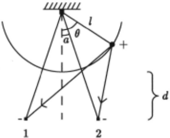
The damped pendulum model presupposes that the force on the bob is independent of the bob's location. The model for the variable attraction between a posi­ tively charged pendulum bob and two negative charges is more complicated (Figure 6). Each negative charge exerts a force

along the line between it and the bob, with a the angle between that line and the pendulum, k the coefficient of electrostatic attraction between the bob and the charge, 1 the length of the arm, and d the vertical distance from the bob's orbit to the line connecting the two negative charges. The two-charge pendulum obeys the equation

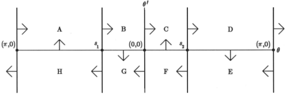
with a the angle between each pole and the vertical, k1 and k2 corresponding to the left and right charges, J-t the damping coefficient, and m the mass of the bob. Figure 7 contains the qualitative dynamics for the case of equal charges (k1 = k2). Saddles appear at (1r,O) and (0, 0) where the charges cancel each other. A sink appears where each charge is strongest. The pendulum can spin (A-B-C-D and E-F-G-H), oscillate around both negative charges (A-B-C-D-E-F-G-H), oscillate around the left charge (A-B-G-H), or oscillate around the right charge (C-D-E-F). It can also switch from spinning to oscillating and from oscillating around both charges to oscillating around either charge.

The sinks are located at the points on the() axis where f(B +a, k1) + f(B- a, k2) = 0. We cannot locate them exactly because the equation has no closed-form solution and because the parameters are subject to measurement error. Instead, we bound each sink within a small region of phase space by numeric simulation or by experimen­ tation. Unlike the sinks, which have zero exit proba­ bilities a priori, the bounding regions can have positive exit probabilities, which must be estimated empirically. One can either incorporate the exit probabilities into the Markov model or shrink the bounding regions until their exit probabilities become negligible. The choice involves a tradeoff between modeling time and analysis time.

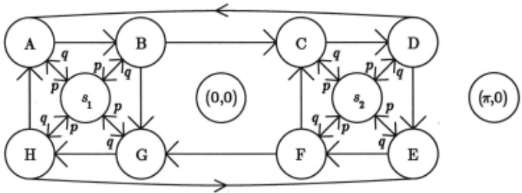
Figure 8 illustrates the first strategy. We assign each bounding region entrance probability p and exit prob­ ability q, assign the saddles zero probabilities, and as­ sume the remaining transitions to be equally likely. The resulting Markov chain consists of three ergodic chains: the two saddles and a primary chain containing all the remaining regions. The asymptotic probabilities of the pendulum being in each region, given that it starts in the primary chain, appear in Figure 9. As q approaches zero, the probabilities of the sinks approach .5 and those of the remaining regions approach zero. The sink prob­ abilities depend only on the ratio pfq; for example given pfq = 10, they are each .37. The second strategy de­ rives the asymptotic probabilities directly by treating s1 and s2 as absorbing states, but incurs the difficulty of constructing regions on which q is negligible.

When the two nearby charges are of unequal mag­ nitude, the unstable equilibria move away from (0, 0) and (1r, 0) and the stable equilibria are positioned asym­ metrically around the ()' axis, but otherwise the qualitative dynamics appears just as in Figure 7. The transi­ tion probabilities, however, change to reflect the greater and lesser attractions of the unequal charges, with entry probabilities p1 and p2 and exit probabilities q1 and q2 . Let P'l and p'f respectively represent the asymptotic probabilities of appearing in states s1 and s2, averaged over all possible transient starting states. For simplic­ ity, we assume that trajectories cannot escape the trap­ ping regions, so that q1 = q2 = 0. Calculating the ratio r 00 = P'l / p'f yields ·

The dependence of r 00 on p1 and p2 agrees with our intuitions. The ratio increases monotonically from 0 as p1 increases from 0 to 1 and decreases monotonically from oo as p2 increases from 0 to 1. It equals 0 when Pl = 0, oo when P2 = 0, and 1 when p1 equals p2.

6 Conclusions and future work

We apply the theory of Markov chains to estimate the likelihoods of possible behaviors of a system, thereby fill­ ing a serious gap in the predictions of qualitative simu­ lation. This theory enables us to draw the best possible conclusions from the available information. We can de­ termine the possible long term behaviors of a system directly from its qualitative dynamics. More detailed information, such as the likelihoods of the possible be­ haviors and the expected settling times for each initial state, require estimates of the transition probabilities be­ tween qualitative states. The estimates can be numeric or symbolic; the analysis is formally identical in both cases, but has O(n 3 ) time-complexity in the former and exponential time-complexity in the latter . We exhibit the utility of our method in several examples, and an­ alyze the robustness of its conclusions to perturbations in the transition probabilities. The likelihoods of the long term behaviors are never sensitive to perturbations in the transition probabilities, whereas the expected set­ tling times can be sensitive.

Our current analysis is only a first step towards full ex­ ploitation of the stochastic approach to qualitative rea­ soning. We have not fully explored the potential of Markov theory. Further investigation may yield sim­ ple ways of determining other qualitative properties of systems through application of known techniques. One might also relax the chain assumption underlying our treatment and instead view the qualitative dynamics as describing a more general Markov process in which tran­ sitions depend on past states. There is a rich theory of these processes which may support many of the same conclusions as above in the more general setting. Incor­ porating global properties of flows, such as energy con­ servation, into stochastic analysis is another topic for fu­ ture research. Finally, automating the model refinement is a major machine learning challenge.

Acknowledgements

We thank Kenneth Yip for valuable suggestions and William Long, Ramesh Patil, Herbert Simon, Peter Szolovits, Michael Wellman, and the referees for help­ ful comments on drafts of this paper.